Machine Learning, Drawn Out
Machine Learning, Drawn Out
An illustrated notebook from vectors to sentence embeddings. This book grew out of a folder of study notes: video frames, pasted articles and one-line reminders collected while learning machine learning from scratch. It retells those ideas in plain English, on one running example, with a picture for nearly every page.
Contents
- 0. How to read this book
- Part I: Vectors, matrices and what they do
- Part II: Neural networks and how they learn
- Part III: Data before the model
- Part IV: Seeing: convolutional networks
- 17. Images as numbers, and the convolution operation
- 18. Kernels, filters, channels and bias
- 19. Why convolution works
- 20. Pooling and strides
- 21. Receptive fields and the visual hierarchy
- 22. 1×1 convolutions, dilation and separable convolutions
- 23. Squeeze-and-Excitation, skip connections, and what CNNs get wrong
- 24. Convolution beyond images
- Part V: Words as numbers: embeddings
- Part VI: Sentences and attention
- Appendix
0. How to read this book
This is a notebook that became a book. The notes it grew from were the usual mess of a learner: screenshots of lectures, whole articles pasted for later, and one-line reminders such as “there is only one parallelepiped”. The mess was useful because it recorded which ideas needed a picture before they made sense. This book keeps that order of discovery and supplies the pictures.
One shop, all the way through. Most chapters use the same example: a small second-hand bookshop that you run. A book on your shelf is a pair of numbers, its page count and its price, and that pair is a vector. Guessing a fair price from the page count is a prediction problem, and it is where bias, variance and cross-validation appear. A photo of a cover is a grid of numbers, and that is where convolutions work. The blurb on the back is a string of words, and that is where embeddings and attention take over. Where an idea is pure geometry, such as a rotation or an eigenvector, the shop steps aside and the picture speaks for itself.
The shape of a chapter. Each chapter opens with two sentences that say what the idea is and why it matters, headed In one breath. The body tells the idea with worked numbers and figures. A box headed From my notes quotes the original reminder, sometimes because it was right, sometimes because it was nearly right and the paragraph after it says what the precise statement is. Watch, read, try lists the videos, articles and interactive pages that the notes had collected, one line each, with the timestamps that were worth saving, together with the papers and reference pages that the chapter’s facts were checked against. Check yourself closes the chapter with two or three questions and their answers.
What the pictures mean. Every figure was drawn by a small program from the same numbers the text uses, so a value you read in a caption is the value the program computed, not a value someone typed. The colours are consistent: blue, orange and green tell categories apart, and a single blue ramp from pale to dark shows magnitude, pale for small and dark for large. Grey is structure: axes, grids and boxes that carry no data. When a figure shows a sequence of steps, read it left to right.
How the parts fit. Part I is the geometry that everything else stands on: vectors, the matrices that move them, determinants, dot products and eigenvectors. Part II builds a neural network from one neuron up and asks how it learns and how learning goes wrong. Part III steps back to the data: what a distribution is, how to recognise one, and how to prepare columns before a model sees them. Part IV is vision: convolutions, receptive fields and the tricks that make image networks work. Part V turns words into numbers, and Part VI turns sentences into numbers you can compare. Read the parts in order the first time; after that, each chapter stands on its own, and the glossary and the note map at the back will take you where you need to go.
Part I: Vectors, matrices and what they do
1. Vectors as arrows and as lists
In one breath. A vector is an arrow that starts at the origin and, at the same time, a short list of numbers saying how far the arrow goes along each axis. Almost everything a machine-learning model reads, from a book’s page count and price to the meaning of a word, arrives as such a list, so the arrow picture is worth owning early.
Picture the shelf of your second-hand bookshop. Each book has a page count and a price, and writing those two numbers in a fixed order describes the book: three hundred pages and two hundred rupees become the pair (300, 200). Counting both in hundreds keeps the numbers small, so the same book is (3, 2). A vector is exactly this, an ordered list of numbers. Each number is a coordinate, and the count of numbers is the dimension; our books live in two dimensions. Order matters, because (2, 3) would be a 200-page book priced at 300 rupees.
The same pair can be drawn. Put the origin, the point (0, 0), where the two axes cross, and draw an arrow from it to the point three steps along the horizontal axis and two steps up. The arrow and the list are two views of one object, and moving between them is the habit this part of the book trains. The list is what a computer stores; the arrow is what your eye can reason about.
Coordinates as shadows
Two arrows deserve names of their own. The unit vector î (say “i-hat”) is one step along the x-axis, the list (1, 0), and ĵ (“j-hat”) is one step along the y-axis, (0, 1). The hat marks a vector whose length is exactly one.
Figure 1.1 reads the book’s coordinates in a second way. Shine a light straight down onto the x-axis and the arrow casts a shadow there, reaching from 0 to 3: the first coordinate. A light shining in from the right casts a shadow of length 2 on the y-axis: the second coordinate. The mathematical name for such a shadow is a projection, the point you reach by dropping straight onto a line, together with its distance from the origin along that line.
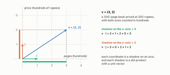 Figure 1.1. The book (3, 2) as an arrow: its shadow on the x-axis (green) is 3 long and its shadow on the y-axis (orange) is 2 long, and the dot products with î and ĵ give the same 3 and 2.
There is also a purely numerical route to the same two numbers. The dot product of two vectors multiplies their matching entries and adds the results. For our book, (3, 2) · (1, 0) = 3 × 1 + 2 × 0 = 3, and (3, 2) · (0, 1) = 3 × 0 + 2 × 1 = 2. The dot product with î picks out the first coordinate and the dot product with ĵ picks out the second. So the shadow picture and the multiply-and-add recipe agree, and here they agree because î and ĵ are one unit long. Chapter 4 shows that the agreement is no accident: for any two vectors, the dot product is one vector’s shadow on the other, multiplied by the other’s length.
Combinations of î and ĵ
Multiplying a vector by a number is called scaling: it stretches the arrow, or flips it round when the number is negative. Adding two vectors means placing the second arrow at the tip of the first and drawing the arrow from the start to the new end; in the list view it means adding the matching entries. With those two moves the book is three copies of î followed by two copies of ĵ, written 3î + 2ĵ. Figure 1.2 draws that walk, and next to it the vector (−1, 2), which takes one step back along î and then two steps up. That second vector is the one chapters 2 and 5 keep asking about.
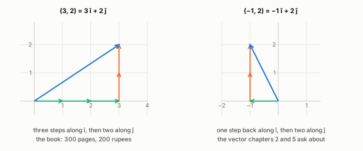 Figure 1.2. Left: (3, 2) is three steps of î and two of ĵ. Right: (−1, 2) is one step backwards along î and two of ĵ. The blue arrow is the sum of the steps.
A sum of scaled vectors such as 3î + 2ĵ is called a linear combination. Every point of the plane is a linear combination of î and ĵ, and in exactly one way, which makes the pair a basis: a set of vectors whose combinations reach every point with none to spare. The arithmetic has a plain meaning in the shop. Two copies of the book are 2 × (3, 2) = (6, 4), six hundred pages for four hundred rupees. The book together with a slim volume (1, 1) makes (3, 2) + (1, 1) = (4, 3): four hundred pages for three hundred rupees.
Nothing changes in more dimensions except the count. A book described by pages, price and age is a vector with three coordinates, an arrow in three-dimensional space, and a third unit vector joins î and ĵ along the new axis. Words in Part V become vectors with a great many coordinates. No one can picture those arrows, yet every rule in this part of the book holds for them unchanged, which is why it pays to learn the rules where they can still be drawn.
From my notes. Ways of thinking about the coordinates of a vector: the projection of the vector on the X axis; the dot product of the vector with î.
Both readings are right, and they agree because î has length one. Measure against a longer arrow along the same axis, 2î for instance, and the dot product doubles while the shadow stays where it was. Chapter 4 turns that detail into the general rule.
Watch, read, try
- Essence of linear algebra — 3Blue1Brown’s sixteen animated chapters; the first four cover this chapter and the next, and later ones return in chapters 3 to 6.
Check yourself. 1. Write a 150-page book priced at 250 rupees as a vector counted in hundreds, and as a combination of î and ĵ. 2. What is (3, 2) · ĵ, and which fact about the book does it pick out? 3. What does the sum (3, 2) + (1, 1) mean for the shop?
Answers. 1. (1.5, 2.5) = 1.5î + 2.5ĵ. 2. It is 2, the price coordinate: two hundred rupees. 3. The two books taken together: (4, 3), four hundred pages for three hundred rupees.
2. Matrices are transformations of the grid
In one breath. A matrix is a compact description of one way to move every point of the plane at once: its columns say where î and ĵ land, and every other point follows from them. Multiplying a matrix by a vector, or two matrices together, is bookkeeping for those moves, and the same bookkeeping runs every layer of a neural network.
A linear transformation is a way of moving every point of the plane so that the origin stays put and the grid lines stay straight, parallel and evenly spaced. Rotations, stretches and shears qualify; bending the plane, or sliding all of it sideways, does not. The rule about grid lines has a strong consequence. Every vector is a combination of î and ĵ (chapter 1), and a linear transformation carries combinations along: a vector that was −1 of î plus 2 of ĵ before the move is −1 of the moved î plus 2 of the moved ĵ after it. So two landing spots, one for î and one for ĵ, decide where everything else goes.
A matrix records those two landing spots side by side, as its columns. Take the matrix A whose first column is (2, 1) and whose second column is (−1, 1). It sends î to (2, 1) and ĵ to (−1, 1); written as a grid of numbers, its first row reads 2, −1 and its second row reads 1, 1. Figure 2.1 shows the whole plane before and after this move. The square grid on the left becomes the slanted grid on the right, still made of straight, parallel, evenly spaced lines.
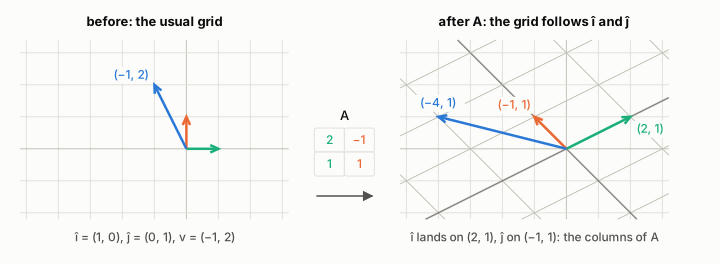 Figure 2.1. The matrix A sends î (green) to (2, 1) and ĵ (orange) to (−1, 1); the whole grid follows, and the vector (−1, 2) lands on (−4, 1).
Matrix times vector
To find where the vector (−1, 2) goes, use its coordinates as amounts of each column: −1 times (2, 1) plus 2 times (−1, 1), which is (−2, −1) + (−2, 2) = (−4, 1). Figure 2.2 draws that sum as two steps taken in the moved grid. The familiar row-by-row recipe gives the same numbers, because each row of the matrix collects one coordinate from every column. Row 1 gives 2 × (−1) + (−1) × 2 = −4 and row 2 gives 1 × (−1) + 1 × 2 = 1. Each row calculation is a dot product, the multiply-and-add recipe of chapter 1, so the same arithmetic has two readings. Read by columns, it combines the landing spots of î and ĵ. Read by rows, it takes one dot product per output coordinate.
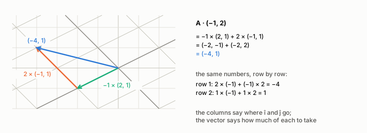 Figure 2.2. A · (−1, 2) as a walk: −1 × (2, 1) in green, then 2 × (−1, 1) in orange, ending at (−4, 1). The row-by-row sums on the right give the same −4 and 1.
This is not a detour from machine learning. A layer of a neural network stores its weights as a matrix and multiplies every incoming vector by it (chapter 7), so everything in this chapter is a picture of what such a layer does to its input.
Matrix times matrix
Doing one move after another is itself a single move, so it has a matrix of its own. Let R be the quarter turn, a rotation by 90° anticlockwise: it sends î to (0, 1) and ĵ to (−1, 0), so those are its columns. Apply A first and R second. The combined matrix is written R·A, with the move that happens first on the right, next to the vector it will meet first. Its columns come from following î and ĵ through both moves. A sends î to (2, 1), and the quarter turn sends (2, 1) to (−1, 2). A sends ĵ to (−1, 1), and the quarter turn sends that to (−1, −1). So R·A has columns (−1, 2) and (−1, −1).
The row-by-column recipe reaches the same matrix mechanically: the entry in row i and column j of a product is the dot product of row i of the left matrix with column j of the right one. The interactive page matrixmultiplication.xyz animates this by turning each column of the right-hand matrix on its side and sliding it down over the rows of the left-hand one. Figure 2.3 is that animation as a filmstrip for R·A.
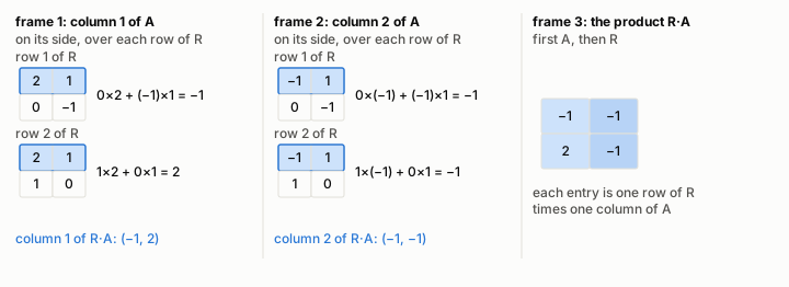 Figure 2.3. Row by column for R·A. Frame 1 lays column (2, 1) of A over each row of R and gets −1 and 2; frame 2 does the same with (−1, 1) and gets −1 and −1; frame 3 is the product, with columns (−1, 2) and (−1, −1).
Order matters. Turning first and then applying A gives A·R, with columns (−1, 1) and (−2, −1), a different matrix. Figure 2.4 puts the two results side by side: the unit square ends up in two different places, although with the same area. Matrix multiplication is therefore not commutative, meaning that swapping the two factors usually changes the answer, even though ordinary multiplication of numbers never minds the order.
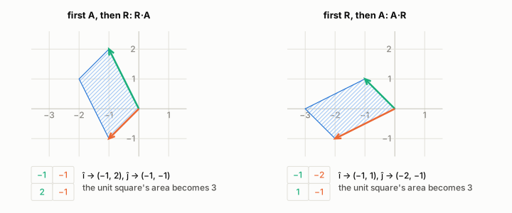 Figure 2.4. First A then R (left) sends î to (−1, 2) and ĵ to (−1, −1); first R then A (right) sends them to (−1, 1) and (−2, −1). Both squares become parallelograms of area 3, in different places.
From my notes. Geometrically, a transformation M translates our grid to someone else’s grid, someone whose unit vectors î and ĵ are the columns of M; numerically, it translates our vectors into the other space.
From my notes. What does (−1, 2) look like to her? What does her vector (x, y) look like to us?
The first note is the right picture, and chapter 5 builds on it: the columns of A are her î and ĵ written in our coordinates. The second note asks two good questions whose answers run in opposite directions, and the video frames saved under the first question in fact answer the second. Multiplying her coordinates (−1, 2) by A gives (−4, 1), which is what her vector looks like to us. The other direction, from our (−1, 2) to her coordinates, needs the move that undoes A, which chapter 3 introduces; she would call our (−1, 2) the pair (1/3, 5/3). Chapter 5 draws both.
Watch, read, try
- matrixmultiplication.xyz — an interactive calculator that animates the row-by-column recipe; type in two small matrices and press Multiply.
Check yourself. 1. Where does the matrix with columns (1, 2) and (3, 0) send the vector (2, 1)? 2. Follow î through R first and then A. Which column of A·R do you get? 3. Why does the row-by-row recipe give the same answer as combining the columns?
Answers. 1. 2 × (1, 2) + 1 × (3, 0) = (5, 4). 2. The quarter turn sends î to (0, 1), and A sends (0, 1) to its second column, (−1, 1); that is the first column of A·R. 3. Each output coordinate adds up that coordinate from every scaled column, and a row of the matrix lists exactly those coordinates, so the row’s dot product with the vector is the same sum.
3. Determinants, inverses and Cramer’s rule
In one breath. The determinant of a matrix is the factor by which its move scales every area, with a minus sign when the move flips the plane over. That one number says whether the move can be undone, and it gives a tidy way, Cramer’s rule, to solve small systems of equations.
A linear transformation turns all the unit squares of the grid into identical parallelograms, so every area in the plane is multiplied by the same factor. That factor, with a sign attached, is the determinant. For a matrix whose rows are a, b and c, d it is ad − bc. The matrix A of chapter 2 has rows 2, −1 and 1, 1, so its determinant is 2 × 1 − (−1) × 1 = 3: the unit square becomes a parallelogram of area 3, and any patch triples in area. Figure 3.1 adds a third matrix S, with rows 1, 2 and 2, 1, whose determinant is 1 × 1 − 2 × 2 = −3.
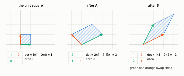 Figure 3.1. The unit square (area 1), its image under A (determinant 3, area 3) and its image under S (determinant −3, area 3, flipped: green and orange have swapped sides).
S also triples areas; the minus sign records something else. Turning anticlockwise from î (green) you reach ĵ (orange) within half a turn, before the move and after A. After S the order is reversed: the plane has been flipped over, as a mirror flips a printed page. A negative determinant marks that flip, and its size still gives the area factor.
When the plane collapses
A determinant of zero multiplies every area by zero: the move squashes the whole plane onto a line, or even onto a single point. Figure 3.2 uses a matrix whose columns, (2, 1) and (4, 2), lie on the same line, so its determinant is 2 × 2 − 4 × 1 = 0. The unit square becomes a thin segment, and different points collide: (2, 0) and (0, 1) both land on (4, 2), and every point of the dashed green line lands on the origin.
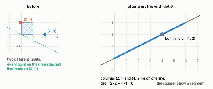 Figure 3.2. A matrix with determinant 0 flattens the plane onto one line: (2, 0) and (0, 1) both land on (4, 2), and the whole dashed line lands on (0, 0).
Collisions make a move impossible to undo. The inverse of a matrix, written A⁻¹, is the move that puts every point back where it started, and it exists exactly when the determinant is not zero. After the collapse in Figure 3.2, a point at (4, 2) cannot say whether it came from (2, 0) or from (0, 1), so no rule can send it back. When the determinant is not zero, the 2 × 2 inverse has a short recipe: swap a and d, change the signs of b and c, and divide everything by the determinant. For A that gives rows 1/3, 1/3 and −1/3, 2/3, which chapter 5 puts to work.
Cramer’s rule, drawn as areas
A system of linear equations is a matrix question in disguise. The pair of equations 3x + 2y = −4 and −x + 2y = −2 asks which vector (x, y) the matrix with columns (3, −1) and (2, 2) sends to (−4, −2). Its determinant is 3 × 2 − 2 × (−1) = 8, not zero, so there is exactly one answer.
Here is the trick. Build a parallelogram on î and the unknown vector (x, y). Its base is î, one unit long, and its height is y, so its signed area is y itself (negative when the vector lies below the axis). Apply the matrix and every area is multiplied by 8, so the moved parallelogram has area 8y. Yet both of its edges are known: î has moved to the first column, (3, −1), and (x, y) has moved to the output, (−4, −2). Its area is the determinant of those two columns, 3 × (−2) − (−4) × (−1) = −10. So 8y = −10 and y = −1.25, as Figure 3.3 draws.
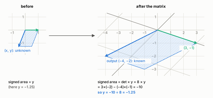 Figure 3.3. Cramer’s rule for y: the parallelogram on î and (x, y) has signed area y; after the matrix its area is −10, and since areas grow by 8, y = −10 ÷ 8 = −1.25.
The same argument with ĵ in place of î finds x: the parallelogram on (x, y) and ĵ has signed area x, and after the move it is built on (−4, −2) and the second column (2, 2), with area (−4) × 2 − 2 × (−2) = −4. So x = −4 ÷ 8 = −0.5 (Figure 3.4). In words, Cramer’s rule replaces one unknown’s column of the matrix by the output, takes the determinant, and divides by the determinant of the original matrix.
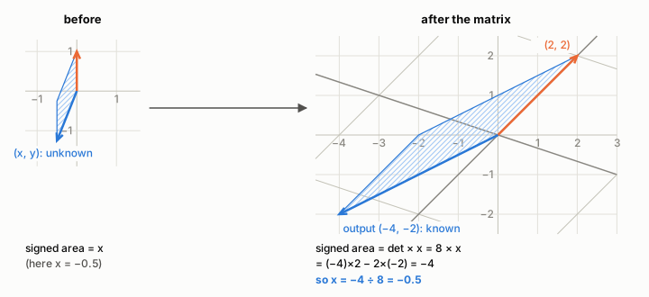 Figure 3.4. Cramer’s rule for x. The parallelogram on (x, y) and ĵ has signed area x; after the matrix its area is −4, so x = −4 ÷ 8 = −0.5.
Volume in three dimensions
Everything carries over to space. A 3 × 3 matrix turns the unit cube into a slanted box called a parallelepiped, whose faces are parallelograms, and its determinant is the factor by which volumes change, again negative for a mirror flip. A slanted box holds its base area times its height, the height being measured straight up from the base, not along the slanted edge. Figure 3.5 shows two boxes with the same 3 by 2 base and height 2; each holds 12.
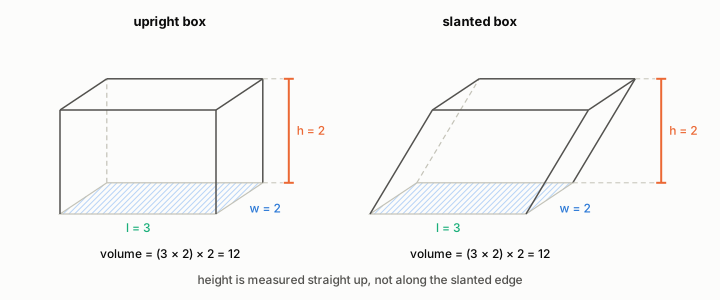 Figure 3.5. An upright box and a slanted box with the same 3 by 2 base and the same height 2 both have volume (3 × 2) × 2 = 12.
From my notes. Why do we need this visual understanding? Because it helps you understand Cramer’s rule easily. Cramer’s rule is not the best way to solve linear equations; Gaussian elimination is faster. The colour coding matters: red and green are the transformation (the coefficients), pink is the contents.
The colour code survives in this book’s palette: green and orange for the matrix’s columns, the coefficients, and blue for the contents, the vector unknown before the move and known after it. The remark about speed needs one refinement. Cramer’s rule takes one determinant per unknown plus one more, which becomes expensive beyond two or three equations; Gaussian elimination, which subtracts multiples of one equation from another until the unknowns come out one at a time, costs about as much as a single determinant. It remains handy for small systems worked by hand.
From my notes. If a transformation moves a point to a new location, the only chance of undoing it is if the transformation has not reduced the dimension of the space. You can’t recover a solid from a plane, or a plane from a line, and you can’t recover anything from a single point.
Duality of determinants: as a transformation, the determinant tells the factor by which area scales; as vectors, the determinant gives the area of the parallelogram (or the volume of the parallelepiped) they form.
Both hold as written: a space that has lost a dimension is the zero-determinant case of Figure 3.2, and the two readings are one fact, since a matrix’s columns are the edges of the shape the unit square or cube becomes.
Watch, read, try
- Cramer’s rule, explained geometrically — 3Blue1Brown’s chapter 12, the source of the area trick in this chapter; the link the notes saved opens at 5:29.
Check yourself. 1. What is the determinant of the matrix with rows 4, 1 and 2, 3, and what happens to a shape of area 2 under it? 2. Why can the matrix with columns (1, 2) and (2, 4) not be undone? 3. Use Cramer’s rule to solve x + y = 3 and x − y = 1.
Answers. 1. 4 × 3 − 1 × 2 = 10, so the shape’s area becomes 20. 2. Its determinant is 1 × 4 − 2 × 2 = 0: it squashes the plane onto a line, and different points land in the same place. 3. The determinant is 1 × (−1) − 1 × 1 = −2. Replacing the first column by (3, 1) gives 3 × (−1) − 1 × 1 = −4, so x = −4 ÷ −2 = 2; replacing the second column gives 1 × 1 − 3 × 1 = −2, so y = 1.
4. Dot products, duality and the cross product
In one breath. The dot product multiplies matching entries and adds them; geometrically it is one vector’s shadow on the other times the other’s length, so its sign says whether two arrows point the same way. The same idea makes a 1 × 2 matrix a vector in disguise and produces the cross product, a vector whose dot product with anything is a volume.
A shadow times a length
Take w = (3, 4) and v = (4, 2). By numbers, v · w = 4 × 3 + 2 × 4 = 20. By geometry, drop a line from the tip of v that meets the line through w at a right angle. The shadow of v on w, from the origin to that foot, is 4 long; w is 5 long, the square root of 3 × 3 + 4 × 4 = 25; and 4 × 5 = 20 again (Figure 4.1).
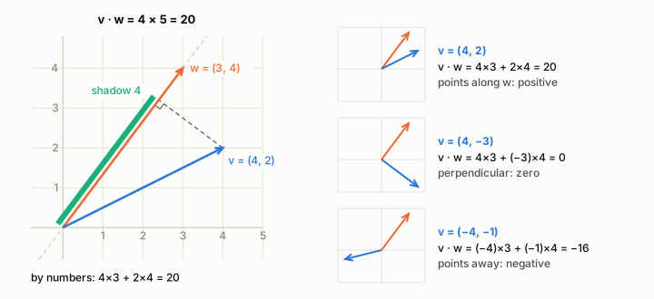 Figure 4.1. Left: v = (4, 2) casts a shadow 4 long on w = (3, 4), which is 5 long: v · w = 20. Right: 20, 0 and −16 as v leans along, across and away from w.
This holds for every pair, either way round. The product is positive when v leans towards w, zero at a right angle, where the shadow shrinks to a point, and negative when v leans away (Figure 4.1, right). In one formula, v · w is the two lengths times the cosine of the angle between them, which is why later chapters compare words with dot products.
A row is a vector in disguise
Now read the recipe the other way. The rule “three times the first coordinate plus four times the second” turns every arrow into one number: a transformation from the plane to the number line, whose matrix is one row with entries 3 and 4, a 1 × 2 matrix. Its outputs for î, ĵ and (4, 2) are 3, 4 and 20, the dot products with (3, 4). A 1 × 2 matrix and a two-dimensional vector are one object seen two ways, a relationship called duality. In Figure 4.2 every point on a dashed line receives the same number, and the number line runs along (3, 4), each number being a shadow on it times 5.
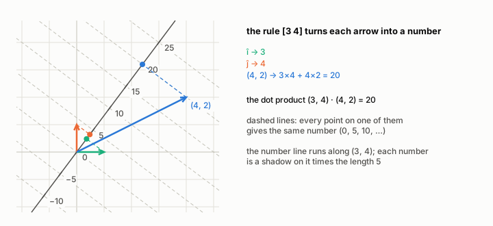 Figure 4.2. The 1 × 2 matrix with entries 3 and 4 sends î, ĵ and (4, 2) to 3, 4 and 20, the dot products with (3, 4).
Moves that keep dot products
The vectors (2, 1) and (1, 2) have dot product 4, and after the quarter turn of chapter 2, (−1, 2) and (−2, 1) still do. After a shear, which slides each row of the grid sideways in proportion to its height, they become (3, 1) and (3, 2), and the dot product jumps to 11 (Figure 4.3). The turn keeps î and ĵ perpendicular and one unit long; the shear tilts ĵ to (1, 1), about 1.41 long. A matrix whose columns are perpendicular vectors of length one is called an orthogonal matrix, and it keeps every length, angle and dot product.
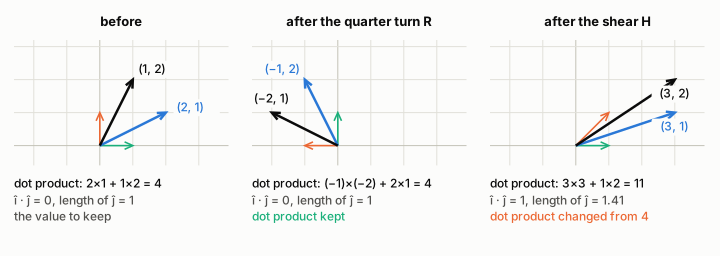 Figure 4.3. The dot product of (2, 1) and (1, 2) is 4 before and after the quarter turn but 11 after the shear.
The cross product as a volume machine
Fix v = (2, 0, 1) and w = (0, 3, 1) and let a third vector x vary. The volume of the box on x, v and w is the determinant with those columns (chapter 3), and it is always the same fixed combination of x’s coordinates. By duality, such a rule is a dot product with one particular vector p: p · x is the volume, whatever x is. That p is the cross product, written v × w.
Base times height gives its geometry. The base is the parallelogram on v and w, the height is how far x reaches straight out of it, and p · x is x’s shadow on p times p’s length. For these to agree for every x, p must stand at right angles to v and w, with length equal to the base area. In Figure 4.4, p = (−3, −2, 6): p · v = 0, p · w = 0, and p is 7 long (9 + 4 + 36 = 49), so the base has area 7. With x = (0, 0, 2) the height is 12 ÷ 7 and the volume 7 × 12 ÷ 7 = 12, the determinant. The right-hand rule picks p’s direction: curl your right hand’s fingers from v towards w and the thumb points along p.
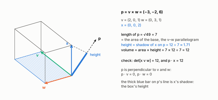 Figure 4.4. The box on x = (0, 0, 2), v and w: base area 7, the length of p = v × w; height 12 ÷ 7, x’s shadow on p; volume 12 = det[x v w] = p · x.
Figure 4.5 shows where p’s three numbers come from.
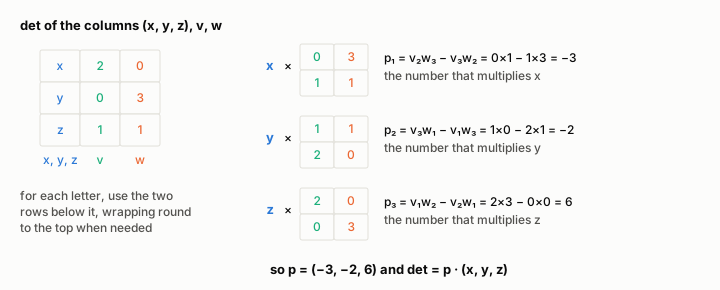 Figure 4.5. Each coordinate of p is a 2 × 2 determinant from the rows of v and w: p₁ = −3, p₂ = −2, p₃ = 6.
From my notes. Dot product is a geometric tool for understanding projections and testing whether vectors point in the same direction; on a deeper level it relates to the transformation represented by one of those vectors. The numeric calculations just appear to be similar.
The dot product of a vector A with itself will always be larger than the dot product of A with any other vector.
PCA / dimensionality reduction: matrix transformations that take 2D to 1D or 3D to 2D. The vector–matrix product and the dot product are the same thing. Projecting v1 on v2 means multiplying the projection of v1 by the magnitude of v2. To find out whether we moved in the direction of the vector or opposite to it, look at the sign of the dot product.
The first note is this chapter’s middle, sharpened once: the calculations are not merely similar but the same, which is what duality means. The second needs a condition, since length counts too: with A = (1, 0) and B = (5, 0), A · B = 5 but A · A = 1. It holds when B is as long as A, by the Cauchy–Schwarz inequality: a dot product never exceeds the product of the two lengths. The third note bridges to dimensionality reduction, describing data with fewer numbers, as Figure 4.2’s matrix does; its middle sentence should say that the dot product is the shadow’s length times the other length. Principal component analysis, chapter 29, chooses the directions.
From my notes. Transformations which preserve the dot product are called orthonormal: rotation, no stretching or squishing. They leave the unit vectors perpendicular and of unit length.
This is the end game of the cross product: given three vectors X, V, W we are looking for a vector P such that P · X = det[X V W], the volume they contain. Important: there is ONLY ONE parallelepiped, formed by our vectors; there is no other.
Both are right. The usual name is orthogonal matrix, orthonormal being accepted too, and the family includes reflections, which flip the plane yet keep every dot product. There is indeed one box, and p depends on v and w alone.
Watch, read, try
- Dot products and duality — 3Blue1Brown’s chapter 9 on the shadow picture and why a row of numbers is a vector.
- Cross products in the light of linear transformations — 3Blue1Brown’s chapter 11, the volume argument of this chapter animated.
Check yourself. 1. Is (2, 1) · (−1, 3) positive, zero or negative, and what does that say about the two directions? 2. Give two vectors A and B for which A · B is larger than A · A. 3. Find (1, 0, 0) × (0, 1, 0) and say which area its length records.
Answers. 1. 2 × (−1) + 1 × 3 = 1, which is positive: the arrows are less than a right angle apart. 2. A = (1, 0) and B = (2, 0): A · B = 2 but A · A = 1. 3. (0, 0, 1); its length, 1, is the area of the unit square on the two vectors.
5. Change of basis
In one breath. The same arrow has different coordinates in different grids, and a matrix whose columns are the other grid’s unit vectors translates one set of coordinates into the other. Describing a move in someone else’s grid is then a three-step sandwich: translate into our words, move, translate back.
Chapter 1 took î and ĵ for granted, but nothing forces everyone to measure with them. Suppose a friend uses her own grid, and her two unit arrows, written in our coordinates, are b₁ = (2, 1) and b₂ = (−1, 1). When she says (−1, 2), she means −1 of b₁ plus 2 of b₂, which in our coordinates is (−2, −1) + (−2, 2) = (−4, 1). Both descriptions name the same arrow in the same place; only the language differs. The list of numbers belongs to a basis, the pair of arrows you measure with, and not to the arrow alone.
The translation is a matrix you have met. Put her basis vectors in as columns and you get A from chapter 2, with columns (2, 1) and (−1, 1). Multiplying her coordinates by A gives ours, exactly as A sent (−1, 2) to (−4, 1) there. The left half of Figure 5.1 shows her grid laid over ours and the two routes to the same point: her two steps along b₁ and b₂, and our single arrow.
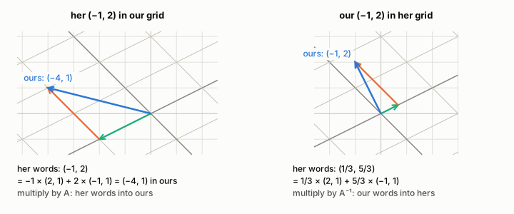 Figure 5.1. Left: her (−1, 2) is −1 × (2, 1) + 2 × (−1, 1) = (−4, 1) in our grid. Right: our (−1, 2) is 1/3 × (2, 1) + 5/3 × (−1, 1), so she calls it (1/3, 5/3).
One point is easy to get backwards. The matrix whose columns are her vectors turns her numbers into ours, not ours into hers. The opposite direction needs the inverse from chapter 3, A⁻¹, with rows 1/3, 1/3 and −1/3, 2/3. Our vector (−1, 2) becomes 1/3 × (−1) + 1/3 × 2 = 1/3 and −1/3 × (−1) + 2/3 × 2 = 5/3, so she calls it (1/3, 5/3). Her own recipe confirms it: 1/3 of (2, 1) plus 5/3 of (−1, 1) is (2/3 − 5/3, 1/3 + 5/3) = (−1, 2). The right half of Figure 5.1 draws this, and it answers the first question of the note in chapter 2.
A move described in her words
Now suppose we want to turn her vector a quarter turn anticlockwise and report the result in her words. Our matrix for the quarter turn, R from chapter 2, expects our coordinates, so it cannot act on hers directly. The fix is a sandwich of three matrices. First A translates her (−1, 2) into our (−4, 1). Then R turns it to (−1, −4). Then A⁻¹ translates back, and she calls the result (−5/3, −7/3). Figure 5.2 lays the three steps out as a pipeline.
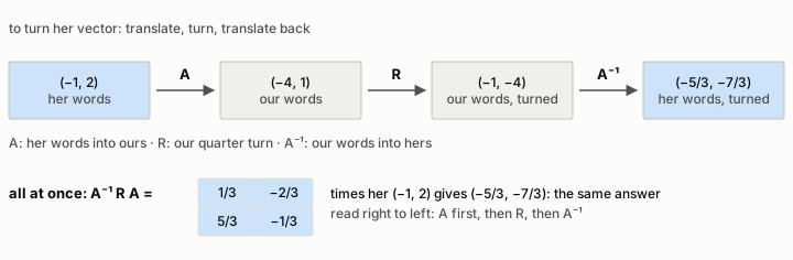 Figure 5.2. Translate, turn, translate back: her (−1, 2) becomes our (−4, 1), turns to (−1, −4) and returns as her (−5/3, −7/3). The single matrix A⁻¹RA, with rows 1/3, −2/3 and 5/3, −1/3, gives the same answer in one step.
Because each step is a matrix, the three can be multiplied into one, written A⁻¹RA and read from right to left: A acts first, then R, then A⁻¹. Its rows are 1/3, −2/3 and 5/3, −1/3, and multiplying her (−1, 2) by it gives (−5/3, −7/3) in one go. This single matrix is the quarter turn as she would write it down. Its columns mean what columns always mean: the first, (1/3, 5/3), is where her first basis vector goes. Her b₁ = (2, 1) turns into our (−1, 2), and that is exactly the vector she calls (1/3, 5/3), as found above. The matrix looks nothing like R, yet it describes the very same motion of the plane. Two matrices related in this way, one equal to A⁻¹ times the other times A, are called similar: they are one transformation described in two bases.
A well-chosen basis can make a transformation look far simpler than it does in ours. Chapter 6 looks for the basis in which a matrix does nothing but stretch along each axis, and principal component analysis, in chapter 29, re-expresses a whole dataset in the basis where its spread is easiest to read. In both cases the arithmetic is the sandwich of this chapter.
From my notes. Change of basis: to see how a transformation of ours affects her vector, first convert her vector to our language, apply the transformation, then convert back: A⁻¹ M A.
That is the whole recipe, and the order of the letters is its one trap: the rightmost matrix acts first, because it stands next to the vector. The note’s first draft wrote the same sandwich in its own notation and named the wrong matrix for the middle step; the transformation in the middle is always ours.
Watch, read, try
- Change of basis — 3Blue1Brown’s chapter 13, where the friend with the other grid is called Jennifer and her basis is the one used here.
Check yourself. 1. Her coordinates are (1, 1). What are ours? 2. Our vector (3, 0): what does she call it? 3. Why does A stand on the right in A⁻¹RA?
Answers. 1. (2, 1) + (−1, 1) = (1, 2). 2. (1, −1), because 1 × (2, 1) − 1 × (−1, 1) = (3, 0). 3. A vector is multiplied by the rightmost matrix first, and her vector must be put into our words before our R can act on it.
6. Eigenvectors and eigenvalues
In one breath. When a matrix moves the plane, most arrows are knocked off the line they lay on, but a few stay on their own line and are only stretched, shrunk or flipped: these are eigenvectors, and each one’s stretch factor is its eigenvalue. Finding them gives a matrix its simplest description, which makes repeated transformations cheap and sits underneath principal component analysis.
Every non-zero vector has a span, its own line: the line through the origin made of all its multiples, and a transformation usually swings a vector off it. Take the matrix M whose columns are (3, 0) and (1, 2). In Figure 6.1 the vector (1, 1) lands on (4, 2), which is not a multiple of (1, 1), but (1, 0) lands on (3, 0), three times itself, and (−1, 1) on (−2, 2), twice itself. Those two stay on their own lines.
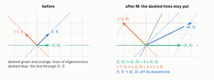 Figure 6.1. Under M, (1, 0) and (−1, 1) stay on their dashed lines, becoming (3, 0) and (−2, 2); the ordinary vector (1, 1) becomes (4, 2), off its line.
A non-zero vector v that a matrix sends to a multiple of itself, Mv = λv, is an eigenvector of the matrix, and the multiple λ (the Greek letter lambda) is its eigenvalue. Every vector on the same line behaves alike, (2, 0) going to (6, 0) and (−3, 3) to (−6, 6), so whole lines of eigenvectors, the dashed green and orange ones, are mapped onto themselves and stretched along their length.
Finding them with a determinant
Write λv as λIv, where I is the identity matrix, the do-nothing transformation with 1s on its diagonal and 0s elsewhere. Then Mv = λv becomes (M − λI)v = 0: the matrix M − λI must send a non-zero vector to zero. By chapter 3 a matrix can do that only when it flattens the plane, when its determinant is zero, so the eigenvalues are the solutions of det(M − λI) = 0.
For our M, M − λI has rows 3 − λ, 1 and 0, 2 − λ, so its determinant is (3 − λ)(2 − λ) − 1 × 0 = (3 − λ)(2 − λ), or λ² − 5λ + 6 multiplied out. Figure 6.2 plots it for λ from 0 to 4, with the parallelogram of the columns of M − λI drawn at five values: its area is 2 at λ = 1, collapses to 0 at λ = 2, comes back flipped with area −0.25 at λ = 2.5, collapses again at λ = 3 and is 2 at λ = 4. The two collapses are the eigenvalues, 2 and 3.
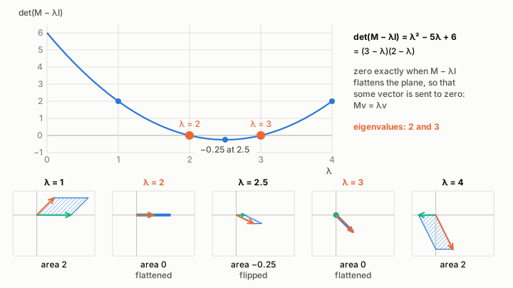 Figure 6.2. det(M − λI) = (3 − λ)(2 − λ) is zero at the eigenvalues 2 and 3 and lowest, −0.25, at 2.5. Below, the parallelogram’s area at λ = 1, 2, 2.5, 3 and 4 is 2, 0, −0.25, 0 and 2.
Each eigenvalue then gives its line. For λ = 3, M − 3I has rows 0, 1 and 0, −1 and sends (x, y) to (y, −y), which is zero only when y = 0: the x-axis. For λ = 2, M − 2I has rows 1, 1 and 0, 0 and sends (x, y) to (x + y, 0), which is zero when x + y = 0: the line through (−1, 1). These are the dashed lines of Figure 6.1.
When there are none
Not every transformation has eigenvectors among the arrows of the plane. The quarter turn R of chapter 2 turns every non-zero vector a quarter turn off its own line; in Figure 6.3 each image meets its vector at a right angle, and every dot product v · Rv is 0. The determinant agrees: R − λI has rows −λ, −1 and 1, −λ, so det(R − λI) = (−λ)(−λ) − (−1)(1) = λ² + 1, which is never smaller than 1. Its solutions are the imaginary numbers i and −i, whose squares are −1: eigenvalues that are complex numbers, not stretch factors of arrows you can draw.
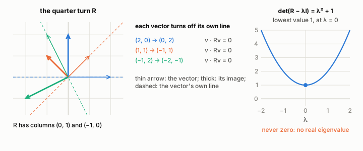 Figure 6.3. The quarter turn sends (2, 0), (1, 1) and (−1, 2) to (0, 2), (−1, 1) and (−2, −1), each at a right angle to its vector; det(R − λI) = λ² + 1 is never below 1.
A shear shows a milder shortage. The shear H of chapter 4, with columns (1, 0) and (1, 1), has det(H − λI) = (1 − λ)², so its only eigenvalue is 1 and its only line of eigenvectors is the x-axis: real eigenvectors, but not two independent lines of them.
The eigenbasis
When a matrix has enough eigenvectors to make a basis, as M does with (1, 0) and (−1, 1), that basis is an eigenbasis, and chapter 5’s sandwich turns M into something plain. Put the eigenvectors as the columns of a matrix P. Then P⁻¹MP, M written in the eigenbasis, is a diagonal matrix, 3 and 2 on its diagonal and zeros elsewhere: in eigen-coordinates M triples the first coordinate, doubles the second, and does nothing else. Figure 6.4 checks this on ĵ, which in the eigenbasis is (1, 1). M sends it to (1, 2), three steps along (1, 0) and two along (−1, 1): eigen-coordinates (3, 2).
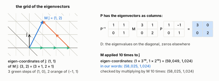 Figure 6.4. In the eigenbasis ĵ = (1, 1) and M ĵ = (3, 2), and P⁻¹MP has 3 and 2 on its diagonal. Ten applications of M give eigen-coordinates (59,049, 1,024), our (58,025, 1,024).
That pays off when a transformation is repeated. Applying M ten times to ĵ takes ten matrix multiplications in our coordinates, but in the eigenbasis only two powers: 3¹⁰ = 59,049 and 2¹⁰ = 1,024 give (59,049, 1,024), which translates back to (58,025, 1,024), the answer the ten multiplications also give. The idea returns in chapter 29: principal component analysis takes the eigenvectors of the covariance matrix, which records how a dataset’s columns vary together, and they point along the directions in which the data spreads.
From my notes. Eigenvectors are the vectors that are unaffected by transformations.
The note is right about direction and too strong otherwise. An eigenvector stays on its own line, but it is still stretched by its eigenvalue: M triples (1, 0) and doubles (−1, 1). Only an eigenvalue of 1 leaves a vector where it was, and a negative one turns it round along the same line.
From my notes. A transformation may not always have eigenvectors, like a rotation by 90°, as it rotates every vector off its own span.
Transformations written in an eigenbasis have an advantage: A⁻¹ M A is a diagonal matrix with the eigenvalues on the diagonal.
Both need one condition. The quarter turn has no real eigenvectors, though its eigenvalues i and −i exist as complex numbers, and some rotations do have real ones: a half turn sends every vector to its opposite, eigenvalue −1. The eigenbasis note holds when the columns of A are eigenvectors, enough of them to form a basis; the shear, with one line of eigenvectors, cannot be made diagonal.
Watch, read, try
- Eigenvectors and eigenvalues, at 11:19 — 3Blue1Brown’s chapter 14; the notes saved this link right after their frames of the quarter-turn example, marked 11:10 and 11:17.
- Eigenvectors and eigenvalues, at 12:30 — the same video, saved beside the eigenbasis reminder; the video’s own summary names the usefulness of an eigenbasis among its topics.
Check yourself. 1. Is (1, 1) an eigenvector of M? Is (−2, 2)? 2. 3Blue1Brown’s other example has columns (2, 1) and (2, 3). What are its eigenvalues? 3. Why can the quarter turn not be written as a diagonal matrix in any basis of real vectors?
Answers. 1. (1, 1) is not: M sends it to (4, 2), which is not a multiple of (1, 1). (−2, 2) is: M sends it to (−4, 4) = 2 × (−2, 2), eigenvalue 2, because it lies on the line through (−1, 1). 2. Its rows are 2, 2 and 1, 3, so det = (2 − λ)(3 − λ) − 2 × 1 = λ² − 5λ + 4 = (λ − 1)(λ − 4): the eigenvalues are 1 and 4. 3. A diagonal description needs a basis of eigenvectors, and the quarter turn has no real eigenvector at all.
Part II: Neural networks and how they learn
7. A neuron, a layer, and why activations must bend
In one breath. A neuron multiplies each input by a weight, adds a bias, and passes the total through a bend called an activation function; a layer is many neurons side by side, which is a matrix times a vector plus a vector. Without the bend, any stack of layers collapses into a single straight-line rule, which is why the hidden layers of a network need non-linear activations.
Suppose you want a machine to help price the books that come into the shop. Give it two facts about each book: its page count in hundreds, x₁, and its age in decades, x₂. A neuron is the smallest unit of a neural network, and it does three things. It multiplies each input by a weight, a number that says how much that input matters and in which direction. It adds the products together with one more number, the bias, which shifts the total up or down whatever the inputs are. The result is the weighted sum, usually written z. Finally it passes z through an activation function, a fixed rule that turns z into the neuron’s output.
Figure 7.1 follows one neuron with weights 0.9 for pages and −1.2 for age, and bias 0.3. The negative weight says that, for this neuron, an older book pushes the sum down. For a 300-page book two decades old, z = 0.9 × 3 + (−1.2) × 2 + 0.3 = 0.6. For a 100-page book of the same age, z = 0.9 × 1 + (−1.2) × 2 + 0.3 = −1.2.
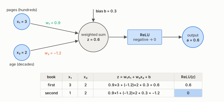 Figure 7.1. One neuron. The first book’s weighted sum is 0.6, which ReLU passes on; the second book’s is −1.2, which ReLU turns into 0. The weight −1.2 itself is untouched.
The activation here is the rectified linear unit, ReLU for short: it returns z when z is positive and 0 otherwise. So the first book’s neuron outputs 0.6 and the second book’s outputs 0. Note carefully what was replaced by zero: the weighted sum, the result of the multiplication, and not any weight. The weight −1.2 stays −1.2 and keeps being adjusted during training.
A layer is several neurons reading the same inputs. Stack their weights as the rows of a matrix W and their biases as a vector b, and the whole layer computes W times the input plus b, then applies the activation to each entry. That is chapter 2’s matrix times vector, followed by a bend.
Why the bend is needed
Suppose we leave the bend out. Figure 7.2 builds a two-layer network whose first layer computes h₁ = x₁ − x₂ and h₂ = 2x₁ + x₂ − 1, and whose second layer computes the output h₁ + 2h₂ + 0.5. Substitute the first layer into the second and the network collapses: the output is 5x₁ + x₂ − 1.5, a single layer with weights 5 and 1 and bias −1.5. For the input (1, 2) both routes give 5.5. The general reason is that a matrix times a matrix is one matrix (chapter 2), so any stack of straight layers is one straight layer, however many you pile up. In the words of James, Witten, Hastie and Tibshirani’s textbook, without a non-linear activation the model “would collapse into a simple linear model”.
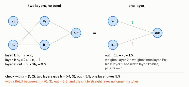 Figure 7.2. Two straight layers equal one: out = 5x₁ + x₂ − 1.5. For x = (1, 2) both give 5.5; with a ReLU between the layers the hidden values become (0, 3) and the output 6.5, which the single straight layer cannot match everywhere.
Put a ReLU between the layers and the story changes. For the same input the hidden values (−1, 3) become (0, 3), and the output is 6.5 instead of 5.5. The network now draws a bent line rather than a straight one, and bends are what let it follow curved relationships.
Four common activations, and what bends buy
Figure 7.3 draws the four activation functions you will meet most. ReLU is 0 for negative inputs and the input itself otherwise. The sigmoid squeezes any number into the range from 0 to 1 along a smooth S, which suits outputs that are probabilities. The hyperbolic tangent, tanh, is a similar S that runs from −1 to 1. The linear activation returns its input unchanged and so does not bend at all.
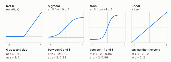 Figure 7.3. ReLU, sigmoid, tanh and linear on inputs from −4 to 4. At z = 2 they give 2, 0.88, 0.96 and 2; at z = −2 they give 0, 0.12, −0.96 and −2.
Figure 7.4 shows what bends buy, on the shop’s price curve, which rises steeply for thin books and levels off for thick ones. Three ReLU units that switch on at 0, 100 and 250 pages add up to a bent line that meets the curve at 0, 100, 250 and 400 pages. More units give more bends and a closer fit; with a non-linear activation, a network with one hidden layer can in principle approximate any reasonable curve.
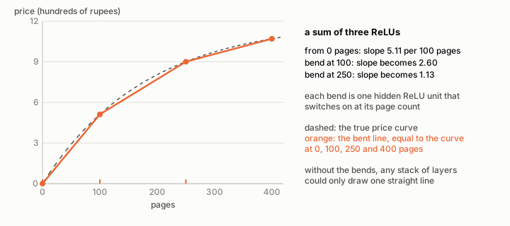 Figure 7.4. Three ReLU units make a line that bends at 100 and 250 pages; its slopes are 5.11, 2.60 and 1.13 hundred rupees per 100 pages, and it meets the price curve at 0, 100, 250 and 400 pages.
The output layer is a different matter. When the network predicts a quantity such as a price, the last neuron is usually left linear, because a price can be any size and a squashing function would cap it. When it predicts a category, the output is squashed into probabilities: a sigmoid for yes or no, or softmax, which turns several scores into probabilities that add up to one, for many classes.
From my notes. Negative weights, which may be the result of the matrix multiplication, are replaced by 0.
The note points at the right place, the result of the matrix multiplication, but names the wrong thing. ReLU replaces negative weighted sums by 0; the weights themselves stay negative when they need to be. In Figure 7.1 the second book’s sum, −1.2, became 0, while the weight −1.2 was never touched.
From my notes. If we use a linear activation in the hidden layers, the hidden layers just compute another linear function of the inputs, so they learn nothing new; it is as if we had no hidden layers. Use a linear activation only in the output layer, when predicting a number.
This one is right, and Figure 7.2 is its proof in numbers. The full note adds a detail worth keeping: with a sigmoid at the output and no bends inside, the whole network is no more capable than logistic regression, which is a single weighted sum passed through a sigmoid. The number meant in the last sentence is a quantity that can take any value, such as a price, and not a count or a class label.
Watch, read, try
- Why Non-linear Activation Functions (C1W3L07) — Andrew Ng’s short lecture from the Deep Learning Specialization, the source of the slide in the note.
Check yourself. 1. A neuron has weights (2, −1), bias −1 and a ReLU. What does it output for the inputs (2, 1) and (1, 3)? 2. One straight layer doubles its input and the next adds 3. What single layer is this, and what does a ReLU between them change? 3. Why is the output neuron of a price predictor usually left linear?
Answers. 1. For (2, 1), z = 4 − 1 − 1 = 2, so the output is 2; for (1, 3), z = 2 − 3 − 1 = −2, so the output is 0. 2. Together they compute 2x + 3. With a ReLU after the doubling, negative inputs give 0 before the 3 is added, so the output is 2x + 3 for x ≥ 0 and 3 for x < 0: a bend at 0. 3. A price can be any size; a sigmoid or tanh would squeeze it into a narrow range.
8. Computation graphs and backpropagation
In one breath. A computation graph breaks a calculation into small steps, each a box that takes a few numbers and returns one. Running it forwards gives the answer; running it backwards and multiplying the local slopes, the chain rule, gives how much the answer moves when each input is nudged, which is exactly what training needs.
Training a network means adjusting its weights so that its error shrinks, and for that you need to know, for each weight, which way and how strongly it pushes the error. That is a derivative: the rate at which an output changes per unit change of one input, measured for very small changes. A network can have hundreds of thousands of weights, so it needs a systematic way to get every derivative at once. The computation graph provides it.
Take the small example from Andrew Ng’s lectures in the note: J = 3(a + bc) with a = 5, b = 3 and c = 2. Break it into steps, each a box that does one thing. The first box computes u = b × c = 6. The second computes v = a + u = 11. The third computes J = 3 × v = 33. Figure 8.1 draws the boxes with arrows pointing the way the values flow; running them left to right is called the forward pass.
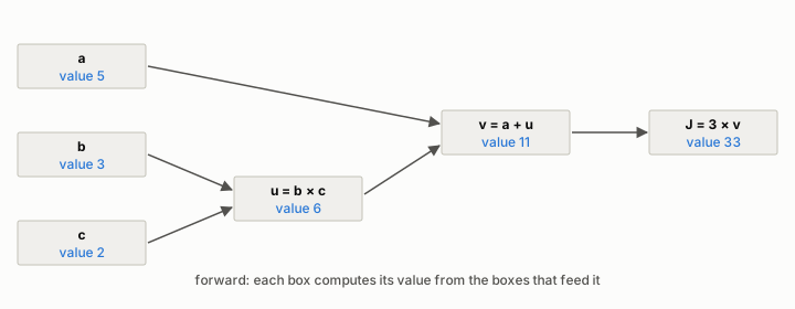 Figure 8.1. The forward pass: a = 5, b = 3 and c = 2 give u = 6, v = 11 and J = 33.
The backward pass
The backward pass gets every slope from one sweep, using local slopes that each box can work out alone. J = 3 × v, so J moves 3 per unit of v. v = a + u, so v moves 1 per unit of a and 1 per unit of u. u = b × c, so u moves c = 2 per unit of b and b = 3 per unit of c. The chain rule says that the slope along a chain of steps is the product of the steps’ slopes: if J moves 3 per unit of v and v moves 1 per unit of u, then J moves 3 × 1 = 3 per unit of u. One step further back, J moves 3 × 2 = 6 per unit of b, 3 × 3 = 9 per unit of c and 3 × 1 = 3 per unit of a. Figure 8.2 runs the graph backwards, from J to the inputs, with the local slope on each arrow and, under each box’s value, its gradient: how far J moves per unit change of that box.
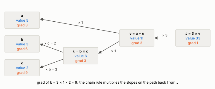 Figure 8.2. The backward pass: gradients 1 for J, 3 for v, u and a, 6 for b and 9 for c. The gradient of b is 3 × 1 × 2 = 6, the product of the slopes on its path back from J.
Checking by nudging
A derivative can also be measured directly, by nudging. Raise b from 3 to 3.001 and run the graph again: u becomes 6.002, v becomes 11.002 and J becomes 33.006. J rose by 0.006 for a nudge of 0.001, six times as much, so J moves at 6 per unit of b, as the backward pass said. Nudging a moves J by 0.003, a slope of 3, and nudging c moves it by 0.009, a slope of 9. Figure 8.3 collects the three experiments. Nudging works, but it costs one extra run of the whole graph for every input, which is hopeless for hundreds of thousands of weights.
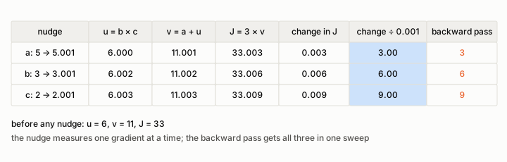 Figure 8.3. Nudging a, b or c by 0.001 moves J to 33.003, 33.006 or 33.009; change ÷ nudge gives 3, 6 and 9, the same as the backward pass.
This is backpropagation: an efficient use of the chain rule that computes the gradient of the output with respect to every input in one backward sweep, one step at a time, reusing each product instead of recomputing it. The gradient here means the whole collection of these slopes, one per input. In a real network J is the error, the inputs whose gradients matter are the weights, and training nudges each weight a little against its gradient to make the error smaller.
Andrej Karpathy’s micrograd shows how little machinery this needs. Its engine is about a hundred lines of Python. Every number in a calculation is wrapped in an object that stores its value, called data, and its gradient, called grad. Each operation that creates a new value also records how to pass gradients back to the values it came from. For a product such as u = b × c, b’s grad receives c times u’s grad and c’s grad receives b times u’s grad, which is the local-slope rule above. Calling backward on the final value visits the graph in reverse order and fills in every grad. One detail in the code matters: gradients are added with +=, so a value that feeds two later boxes collects a contribution from each path.
From my notes. Grads: Computation graphs; Derivatives with computation graphs; Andrej Karpathy, backpropagation.
Those three titles are a good order in which to watch, and this chapter follows it: draw the graph, run it backwards, then see an engine that does it for any graph. The note spelled the third author’s first name “Andrew”; the video is by Andrej Karpathy.
Watch, read, try
- Computation Graph (C1W2L07) — Andrew Ng draws a calculation as boxes and runs it forwards.
- Derivatives With Computation Graphs (C1W2L08) — the same kind of graph run backwards to get its derivatives.
- The spelled-out intro to neural networks and backpropagation: building micrograd — Andrej Karpathy builds a small engine in which every value carries its own gradient.
Check yourself. 1. With a = 5, b = 3 and c = 2, what is J when c is nudged to 2.001, and what slope does that show? 2. Using the chain rule, what is the gradient of J with respect to u? 3. Why does backpropagation beat nudging for a network with many weights?
Answers. 1. u = 6.003, v = 11.003 and J = 33.009; J rose by 0.009, a slope of 9. 2. 3 × 1 = 3. 3. One backward sweep gives every gradient at once, while nudging needs a separate run of the whole network for each weight.
9. Bias, variance and the sweet spot
In one breath. A model that is too rigid misses the real pattern, which is called bias, and a model that is too flexible chases the noise in its training data and changes wildly from one dataset to the next, which is called variance. The best model sits between the two, and the only way to find it is to test on data the model has not seen.
Back in the shop, you would like a rule that prices a book from its page count alone. For this chapter we invent the truth, so that every model can be checked against it: a book with $x$ pages is worth $12\,(1 - e^{-x/180})$ hundred rupees, a curve that climbs steeply for thin books and levels off towards 12 for thick ones. All prices in this chapter and the next are in hundreds of rupees. Real prices wobble around such a curve for reasons no rule can see, so each of our books gets a small fixed wobble. The eight books used to fit models form the training set; eight more books with the same page counts and different wobbles form the test set, kept back to judge the models.
| pages | true price | training book | test book |
|---|---|---|---|
| 60 | 3.40 | 4.00 | 3.00 |
| 90 | 4.72 | 4.22 | 5.42 |
| 120 | 5.84 | 6.64 | 5.24 |
| 160 | 7.07 | 6.17 | 7.57 |
| 200 | 8.05 | 8.45 | 7.25 |
| 260 | 9.17 | 8.47 | 9.47 |
| 320 | 9.97 | 10.47 | 9.47 |
| 400 | 10.70 | 10.40 | 11.30 |
Figure 9.1 fits two models to the training books. The first is a straight line chosen by least squares: of all straight lines, the one whose squared vertical misses add up to the smallest total. The second is a polynomial of degree 7. The degree of a polynomial is its highest power, and each extra degree allows one more bend, so a degree-7 curve can bend six times and, with eight books, pass through every one of them.
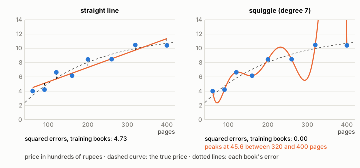 Figure 9.1. On the training books the straight line’s squared errors add up to 4.73 and the squiggle’s to 0.00; between 320 and 400 pages the squiggle climbs off the chart to 45.6.
On the training books the squiggle is perfect: its squared errors total 0.00, against 4.73 for the line. On the test books the order flips, as Figure 9.2 shows. The line’s squared errors total 4.63, much as in training, while the squiggle’s jump to 10.61. Between 320 and 400 pages, where no book held it down, the squiggle climbs as high as 45.6, over four thousand rupees for a book of about 375 pages.
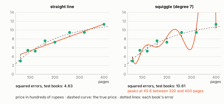 Figure 9.2. On the test books the straight line’s squared errors total 4.63 and the squiggle’s 10.61.
Bias and variance
The two failures have names. Bias is the error that comes from approximating a complicated relationship by a model too simple to follow it. The straight line cannot bend, so it overprices the thinnest book (4.51 against a true 3.40) and the thickest (11.36 against 10.70) and underprices the middle (7.33 against 8.05 at 200 pages), and more data would not cure that. Variance is how much a fitted model would change if it were fitted to a different set of training books. Fit both models again, this time to the eight test books as though they were the training set. The line barely moves: its slope goes from 2.02 to 2.20 hundred rupees per 100 pages. The squiggle changes out of recognition: at 360 pages the version fitted to the training books predicts 38.3, while the version fitted to the test books predicts −13.6, a negative price.
A model that scores well on its training data and badly on new data is overfitting: it has learned the wobbles as though they were the pattern. James, Witten, Hastie and Tibshirani add a useful precision in their textbook: a model is overfitting when a less flexible one would have done better on the test data.
The sweet spot
Figure 9.3 fits polynomials of every degree from 0 to 7 and measures the mean squared error, the average of the squared misses, on both sets of books. The training error falls at every step, from 5.55 for a flat line (degree 0) to 0.00 at degree 7. The test error falls from 6.47 to 0.38 at degree 2, then climbs back to 1.33. Degree 2 is the sweet spot for these books: flexible enough to follow the curve, stiff enough to ignore the wobbles.
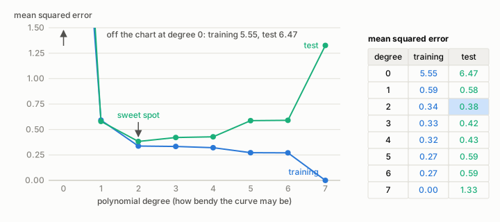 Figure 9.3. Training error (blue) falls from 5.55 to 0.00 as the degree rises; test error (green) is lowest, 0.38, at degree 2 and rises to 1.33 at degree 7.
This shape, training error always falling and test error falling then rising, is the bias–variance trade-off. The expected test error of a method splits into three parts: the variance of its fit, the square of its bias, and noise that no model can predict. More flexibility lowers the bias and raises the variance, and the sweet spot is where their sum is smallest; the noise sets a floor that no model gets under. Three families of methods help find the spot, and a StatQuest frame saved in the note names them: regularisation, which charges a model for complexity (chapter 11 is an example); bagging, which fits many models to resampled copies of the data and averages them, cutting variance; and boosting, which fits models one after another, each to the errors the previous ones left.
From my notes. Blue is the true relationship, red is the predicted one.
The frames the note saved use those colours. This book’s figures keep the roles and change the palette: the true curve is dashed grey and the fitted models are orange.
From my notes. Variance is observed across different datasets. Blue is the training set, green the test set.
The dots keep the note’s colours, blue for training and green for test. And variance is indeed about different datasets: it only shows when the same method is fitted to more than one, as in the refit above, which is why a training error alone can never reveal it.
Watch, read, try
- Machine Learning Fundamentals: Bias and Variance — Josh Starmer’s StatQuest introduction to bias, variance and overfitting.
Check yourself. 1. A model has training error 0.1 and test error 3.0. Is its main problem bias or variance? 2. Why can the straight line not reach zero training error on the eight books? 3. In Figure 9.3, which degree would you choose, and why not the one with the lowest training error?
Answers. 1. Variance: it fits the training data closely and new data badly, the signature of overfitting. 2. The books do not lie on one straight line, because the true relationship curves and each book has its own wobble, and a line has only two numbers to adjust. 3. Degree 2, which has the lowest test error, 0.38; degree 7 reaches zero training error only by passing through every training book, wobbles included.
10. Cross-validation
In one breath. Cross-validation estimates how well a method will do on new data by holding back one slice of the data at a time, training on the rest and testing on the held-back slice, until every slice has been tested once. The average of those test scores lets you compare methods and choose settings without locking away a large test set that never helps training.
Chapter 9 had the luxury of eight extra books kept purely for testing. Usually there is one pile of data, and every book hidden for testing is a book the model cannot learn from. Nor can a model be judged on the books it was trained on, because the training error flatters it, as the squiggle showed. The simplest compromise, called the validation-set approach, splits the pile once into a training part and a testing part. It has two weaknesses: the verdict depends on which books happened to land in each part, and the model learns from only some of the data.
Cross-validation removes both weaknesses. Put all sixteen priced books from chapter 9 into one pile, sort them by page count and deal them into four blocks like cards: the first book to block 1, the second to block 2, and so on round again. Figure 10.1 shows the four rounds that follow. In round 1, block 1 is held back, the method is trained on the other three blocks, and the trained model is scored on block 1. Round 2 holds back block 2, and so on. After four rounds every book has been tested exactly once, by a model that never saw it, and the method’s score is the average of the four test errors. This is four-fold cross-validation, and each block is called a fold.
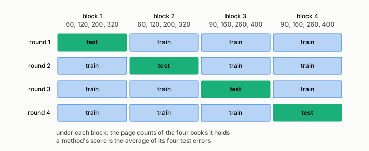 Figure 10.1. Sixteen books dealt into four blocks. Each round tests one block (green) with a model trained on the other three (blue), so every book is tested exactly once.
Because the method is retrained in every round, cross-validation scores a method, a recipe for fitting, rather than one fitted model. Figure 10.2 is the scoreboard for five recipes, polynomials of degree 1, 2, 3, 5 and 7. The straight line averages 0.90; the gentle curve of degree 2 averages 0.63, the best; degree 3 averages 0.68, degree 5 averages 0.81 and the squiggle 1.33. The verdict agrees with chapter 9’s test set without needing one. Look at rounds 2 and 4, though: there degree 3 edges out degree 2, by 0.63 against 0.65 and 0.61 against 0.62. A single split could have crowned the wrong method, and the average over all four rounds is steadier. Once the winner is chosen, it is fitted again on all sixteen books.
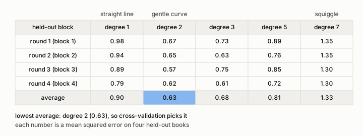 Figure 10.2. The scoreboard: average test errors of 0.90, 0.63, 0.68, 0.81 and 1.33 for degrees 1, 2, 3, 5 and 7. Degree 2 wins on average, though degree 3 wins rounds 2 and 4.
The scores of one method also move from round to round, a reminder that the average is an estimate with its own spread, not a fixed property of the method. Degree 2’s four scores run from 0.57 to 0.67. Their standard deviation, the typical distance of a score from its average, is 0.043, and dividing it by the square root of the number of rounds gives the standard error of the average, 0.022. James, Witten, Hastie and Tibshirani describe a rule for close calls: choose the simplest method whose average lies within one standard error of the lowest. Here degree 1, the only simpler candidate, averages 0.90, far above 0.63 + 0.022 = 0.652, so the rule keeps degree 2. When two methods do land inside that band, the rounds cannot tell them apart, and the simpler one is the safer choice. Dealing the books into different blocks would also shift every score a little, which is why cross-validation is sometimes repeated with several shuffles.
How many folds
The number of blocks is a choice. With k folds, each round trains on all but one k-th of the data and the method is fitted k times. In practice five or ten folds are the usual choice, and a StatQuest frame saved in the note calls ten blocks very common. At the extreme, leave-one-out cross-validation holds back a single book in each round, which for our pile would mean sixteen rounds; it wastes no data but costs one fit per book, which grows expensive when there are many books or the method is slow to fit.
Choosing settings and methods
Many methods have a tuning parameter, a setting that is not learned from the data but chosen beforehand, such as the degree of the polynomial here or the penalty λ of ridge regression in chapter 11. Cross-validation chooses it the same way it chooses between methods: try several values, score each by its average test error, and keep the best. When the answers are categories rather than numbers, the score of each round can be the count of test items labelled correctly, which is how the StatQuest example compares three classification methods.
One caution keeps the scores honest. Every step that learns from the data, including the choice of which inputs to use, has to be carried out inside each round on the training blocks alone. If the held-back block helped make those choices, it is no longer new data, and the score flatters the method.
Watch, read, try
- Machine Learning Fundamentals: Cross Validation — StatQuest’s walk through four-fold and ten-fold cross-validation and its use for comparing methods and tuning parameters.
Check yourself. 1. With 20 books and five-fold cross-validation, how many books train each model, how many test it, and how many models are fitted? 2. What would leave-one-out cross-validation mean for our sixteen books? 3. Why fit the chosen method again on all the data at the end?
Answers. 1. Sixteen train and four test in each round, and five models are fitted. 2. Sixteen rounds, each training on fifteen books and testing on the one left out. 3. The rounds were only for choosing; the final model should learn from every book available.
11. Ridge regression: a little bias for a lot less variance
In one breath. Ridge regression fits a line by keeping the usual sum of squared misses small while also charging a penalty, λ times the slope squared, so it prefers flatter lines. When data are scarce, this deliberate bias buys a large drop in variance, and cross-validation decides how much penalty to charge.
Suppose a new series arrives at the shop and you have priced only two of its books: 100 pages at 200 rupees and 300 pages at 500 rupees, the points (1, 2) and (3, 5) when both are counted in hundreds. Least squares draws the line through both, y = 0.5 + 1.5x, where x is the page count and y the price. It misses nothing, so its training error is zero. But two books are a thin basis for a pricing rule, and a line that steep, charging 150 rupees for every extra 100 pages, may say more about these two books than about the series.
Ridge regression changes what counts as a good line. Its cost is the sum of squared misses plus a penalty, λ times the slope squared, where λ (the Greek letter lambda) is a number we choose, zero or more. The intercept, the height at which the line crosses the price axis, is not penalised, because it only sets the general level of prices. With λ = 0, ridge regression is ordinary least squares. With λ = 1, compare two candidates, as in Figure 11.1. The least-squares line pays nothing for misses but 1 × 1.5² = 2.25 in penalty. The line y = 1.5 + x misses each book by 0.5, costing (−0.5)² + 0.5² = 0.5, and pays a penalty of 1 × 1² = 1, a total of 1.5, the lowest cost any line can reach at this λ.
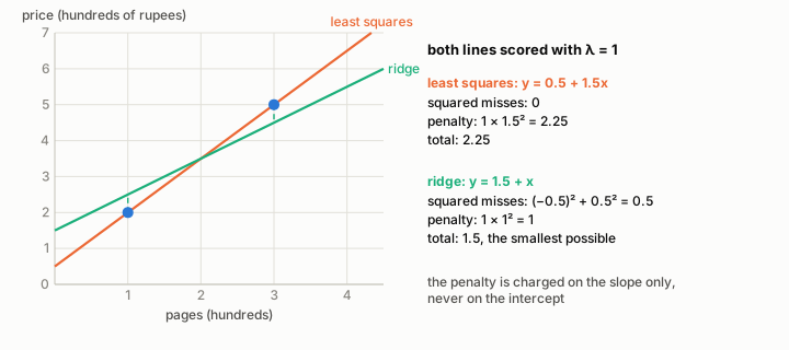 Figure 11.1. With λ = 1, the least-squares line y = 0.5 + 1.5x costs 0 + 2.25 = 2.25, and the ridge line y = 1.5 + x costs 0.5 + 1 = 1.5, the cheapest possible.
Where does y = 1.5 + x come from? For any slope, the best intercept puts the line through the average book, (2, 3.5), so the cost depends on the slope alone. Figure 11.2 plots that cost against the slope for three values of λ. With no penalty the lowest point sits at slope 1.5; with λ = 1 it moves to 1; with λ = 3 it moves to 0.6. For these two books the best slope works out as 3 divided by (2 + λ), so a larger penalty always gives a flatter line, and a very large one flattens it to the average price.
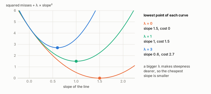 Figure 11.2. Cost against slope, with the best intercept for each slope: the lowest points sit at slopes 1.5, 1 and 0.6 for λ = 0, 1 and 3, with costs 0, 1.5 and 2.7.
Does the flatter line predict better?
Only new books can say. Six more books from the series arrive, and in this invented example their prices follow a gentler trend than the first two books suggested. Figure 11.3 lays both lines over them. The least-squares line misses them by a total squared error of 4.69; the ridge line for λ = 1 misses by only 0.64, and the line for λ = 3 happens to score 0.64 as well. The two training books sat steeper than the trend, and the penalty stopped the line from believing them completely. That is the trade in this chapter’s title: a little bias, since ridge no longer fits the training books exactly, for a large drop in variance, since the line no longer swings with every accident of the training data.
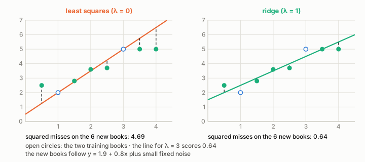 Figure 11.3. On six new books the least-squares line’s squared misses total 4.69 and the ridge line’s (λ = 1) total 0.64.
The slope is also the model’s sensitivity: how far the prediction moves when the input moves by one unit. Figure 11.4 draws a step of one unit, 100 pages, on each line. The least-squares line raises its predicted price by 1.5, the λ = 1 line by 1 and the λ = 3 line by 0.6. A flatter line passes on less of any change, or any error, in its input.
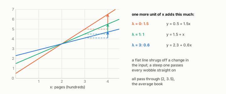 Figure 11.4. One more unit of pages raises the prediction by 1.5, 1 and 0.6 for λ = 0, 1 and 3; all three lines pass through the average book (2, 3.5).
Choosing λ, and a close relative
Nothing in the method says which λ to use. It is a tuning parameter, and chapter 10’s cross-validation chooses it: try a range of values, score each by its average test error across the folds, and keep the best. With many inputs, ridge regression charges λ times the sum of all the squared slopes. Because that charge depends on the units each input is measured in, the inputs are usually standardised first, rescaled so that each has the same spread. Its close relative, the lasso, charges λ times the sum of the slopes’ sizes, ignoring their signs, instead of their squares. That small change has a large effect: the lasso can push some slopes exactly to zero, dropping those inputs from the model altogether, which ridge regression does not do.
From my notes. The penalty added to the error is λ × m², where m is the slope.
From my notes. When the slope of the line is small, predictions are much less sensitive to changes in the input.
Both are right. The first is the ridge penalty for a single input; with several inputs it becomes λ times the sum of the squared slopes, still leaving the intercept alone. The second is Figure 11.4 in one sentence, and it echoes the StatQuest frame the note saved under its heading.
Watch, read, try
- Regularization Part 1: Ridge (L2) Regression — StatQuest’s introduction to ridge regression and its penalty on the slope.
Check yourself. 1. For our two books and λ = 2, which slope and intercept does ridge regression choose? 2. What happens to the ridge line as λ grows very large? 3. Why is the intercept left out of the penalty?
Answers. 1. Slope 3 ÷ (2 + 2) = 0.75 and intercept 3.5 − 2 × 0.75 = 2, so y = 2 + 0.75x. 2. The slope shrinks towards 0 and the line flattens towards the average price, 3.5, that is 350 rupees. 3. The intercept only sets the general level of prices; shrinking it would drag every prediction towards zero without making the line any less sensitive to its input.
Part III: Data before the model
12. Distributions: PMF, PDF, CDF
In one breath. A probability distribution lists the values a quantity can take and how likely each one is. Counts are described by a probability mass function, measurements by a probability density function, and both by a cumulative distribution function, the tool behind medians, percentiles and most of the plots in the next three chapters.
Two questions come up in the shop every day. How many books will the next customer buy, and how long is the next book that comes through the door? The first answer is a whole number: one book, two books, never two and a half. The second is a length, and a book can have almost any number of pages, so we treat the page count as a measurement on a continuous scale even though pages come in whole numbers. A quantity that can only take separate, countable values is called discrete. One that can take any value in a range is called continuous. The two kinds are described in slightly different ways, and mixing them up causes a surprising amount of confusion.
Discrete: a probability for every value
Suppose you count the baskets of 40 customers. Fourteen buy one book, eleven buy two, seven buy three, four buy four, and two customers each buy five and six. Dividing every count by 40 gives the probability mass function, or PMF: the probability of each possible value. Figure 12.1 draws it as six bars.
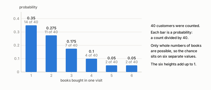 Figure 12.1. The probability mass function of books bought per visit. Each bar is a count divided by 40; the six heights add up to exactly 1.
Two rules hold for every PMF. Each probability lies between 0 and 1, and together they add up to exactly 1, because every customer buys some number of books. Reading a PMF is direct: the chance that a customer buys two books is the height of the second bar, 0.275.
Continuous: probability as area
Page counts need a different picture. To have one, the program that draws this book’s figures produced a sample of 60 page counts from a known curve, using a fixed random-number generator so that every figure sees the same 60 books. The curve is a lognormal distribution: a quantity whose logarithm follows the bell-shaped normal curve. Ours has a median of 240 pages, so half of all books are shorter and half longer, and a spread of 0.45 on the logarithmic scale, written σ.
For a continuous quantity there are so many possible values that the chance of hitting any one exact value is zero. What has a probability is an interval. The probability density function, or PDF, is a curve drawn so that the area under it between two values equals the probability of landing between them. Figure 12.2 shades the area between 200 and 300 pages. It comes to 0.347, so roughly a third of all books have 200 to 300 pages.
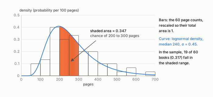 Figure 12.2. A probability density. The shaded area under the lognormal curve between 200 and 300 pages is 0.347; in the sample, 19 of the 60 books (0.317) fall in that range.
The height of the curve is not a probability. It is a density, a probability per unit of length, which is why the axis of Figure 12.2 reads “probability per 100 pages”. The curve peaks at about 0.41 per 100 pages near 196 pages, and that number becomes a probability only after it is multiplied by a width. The sample wobbles around the curve: 19 of the 60 books fall between 200 and 300 pages, a fraction of 0.317, a little below the curve’s 0.347. A sample is always a noisy copy of its distribution, and chapter 13 is about working backwards from such a copy to the curve.
Cumulative: adding up from the left
Often the useful question is not how likely a value is, but how likely it is to be that value or less. The cumulative distribution function, or CDF, answers it. Written F(x), it is the probability that the quantity is at most x. For a discrete quantity the CDF is a running total of the PMF, so it climbs in steps: the chance that a customer buys at most four books is 0.35 + 0.275 + 0.175 + 0.1 = 0.9, marked on the left of Figure 12.3. For a continuous quantity the CDF is the area under the density to the left of x, so it rises smoothly. The lognormal curve says that 0.690 of all books have at most 300 pages. The blue staircase on the right of Figure 12.3 is the sample’s own CDF, which climbs by one sixtieth at each book; at 300 pages it has reached 38 of 60, or 0.633.
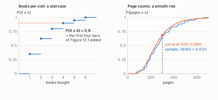 Figure 12.3. Two cumulative distribution functions. Left, books bought: P(X ≤ 4) = 0.9, the first four bars of Figure 12.1 added. Right, page counts: the curve gives 0.690 at 300 pages and the sample 38/60 = 0.633.
Read backwards, the CDF gives quantiles: the value below which a chosen fraction of the data falls. The median is the 0.5 quantile, 240 pages for our curve, and the 25th percentile is the 0.25 quantile. The NIST/SEMATECH handbook calls this inverse of the CDF the percent point function. Quantiles return twice in this part of the book: in chapter 13 they compare a sample with a model, and in chapter 15 they make several samples comparable.
From my notes. PMF is for discrete variables: it tells us the probability of each value. PDF is for continuous variables.
The note draws the line between the two in the right place. In the original, the PDF heading went on to promise the probability of each continuous value, and that half needs adjusting: a density gives probability per unit, the probability of any exact value is zero, and only an area under the density is a probability.
Watch, read, try
- Probability Distribution Functions (PMF, PDF, CDF) — zedstatistics on the three functions.
Check yourself. 1. Is the number of books on a shelf discrete or continuous, and which function describes its probabilities? 2. From Figure 12.1, what is the chance that a customer buys more than four books? 3. The density in Figure 12.2 peaks at about 0.41 per 100 pages near 196 pages. Does that mean 41% of books have exactly 196 pages?
Answers. 1. Discrete, because it takes whole-number values only; a probability mass function describes it. 2. 1 − 0.9 = 0.1, which is the last two bars, 0.05 + 0.05. 3. No. A density is a probability per unit of length; in the continuous model the chance of exactly 196 pages is zero, and a probability needs an interval, such as 0.347 for 200 to 300 pages.
13. Which distribution does my data follow?
In one breath. Many methods assume a shape for the data, so before trusting them it pays to find out which distribution a sample resembles. The routine is short: look at the histogram, test a shortlist, read the probability plots, and keep the simplest shape that fits.
Here we pretend not to know that chapter 12’s page counts came from a lognormal curve, and recover it with the steps of Jim Frost’s article in my notes.
Look before you test
Start with a histogram (Figure 13.1). The page counts pile up between 150 and 300 and trail off as far as 658, so the distribution is skewed right: its long tail points towards large values. Data that press against a hard limit tend to spread away from it, and no book has fewer than zero pages.
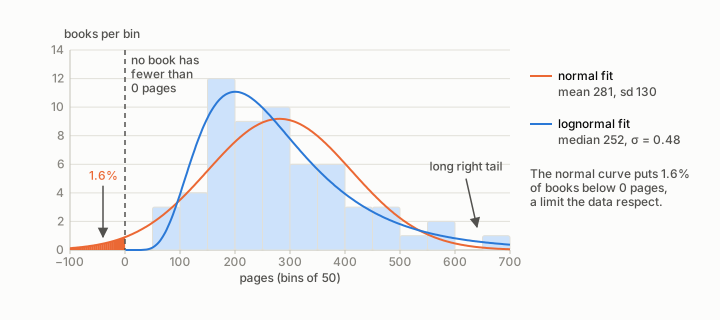 Figure 13.1. The 60 page counts with two fitted curves. The normal curve (mean 281, sd 130) misses the peak and puts 1.6% of books below zero pages; the lognormal (median 252, σ = 0.48) follows the bars and the long right tail.
The normal curve with the sample’s mean and standard deviation misses the peak and gives 1.6% of books fewer than zero pages; the lognormal follows the bars. Two humps would suggest two kinds of book mixed together; ours has one.
Test, and read the p-value backwards
A goodness-of-fit test asks whether the sample could have come from a stated distribution. Its null hypothesis is that it did, so a small p-value rejects the candidate; unusually, the hoped-for result is a high one. The Anderson–Darling test compares the sample’s staircase CDF with the fitted one, weighting the tails more than the Kolmogorov–Smirnov test, another common fit test, does, and its statistic A² grows as the fit worsens.
| candidate | A² | p-value |
|---|---|---|
| normal | 1.11 | 0.006 |
| lognormal | 0.25 | 0.74 |
| gamma | 0.23 | needs its own table |
| Weibull | 0.59 | needs its own table |
The normal is rejected: 0.006 is far below 0.05, and its adjusted A² of 1.12 exceeds 0.752, the 5% critical value in the NIST/SEMATECH handbook. The lognormal, tested through the logarithms of the page counts, gives 0.74 and stays. The gamma and Weibull, two more right-skewed families, need p-value tables of their own, so their A² values and plots decide. Each family here has two parameters, numbers that pin the curve down. Some families add a third, a threshold or smallest possible value, and Frost’s tables then show LRT P, a likelihood-ratio test of whether it earns its place. Counts and categories take a chi-square test instead.
Plot: the fat-pencil test
A probability plot, or Q–Q plot (quantile against quantile), puts each book’s real page count against the count the fitted model expects at that rank (the NIST handbook uses the model’s order-statistic medians). A good model gives a straight line, and Frost’s informal fat-pencil test asks whether a fat pencil laid along it would hide the dots.
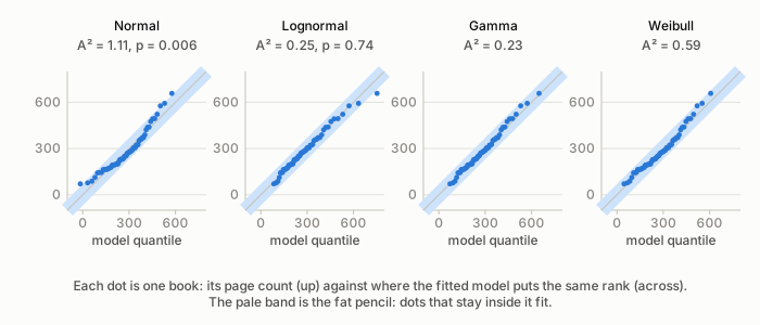 Figure 13.2. Probability plots against four fitted distributions. The normal panel bends upward at both ends; the lognormal and gamma panels stay inside the pale band, the fat pencil; the Weibull panel curls a little at the top.
In Figure 13.2 the normal panel’s dots sit above the line at both ends and below it in the middle, the mark of a right skew. The lognormal and gamma panels are straight, and the Weibull curls slightly at the top. Plots matter most for large samples, where a test can reject a distribution over a trivial departure; as an answer on Cross Validated notes, no real sample follows any distribution exactly.
A threshold, and knowing when to stop
Use a threshold only when the subject supplies a real floor, as it does for books on paper: UNESCO’s 1964 recommendation on book statistics counts only publications of at least 49 pages, cover excluded. Figure 13.3 fixes a threshold there, but our shortest book has 71 pages and A² worsens from 0.25 to 0.79, so two parameters are enough.
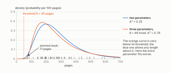 Figure 13.3. A threshold at 49 pages, UNESCO’s floor for a book. The three-parameter curve is zero below the threshold, but the shortest book has 71 pages and A² worsens from 0.25 to 0.79, so two parameters are enough.
The fitted median and spread, 252 and 0.48, are near the true 240 and 0.45; 60 books are only a sample. The gamma fits about as well; no test on 60 books can separate them, so subject knowledge or convenience decides. Box–Cox and Johnson transformations bend data until they look normal; they do not say what shape the data have. Figure 13.4 gathers the route.
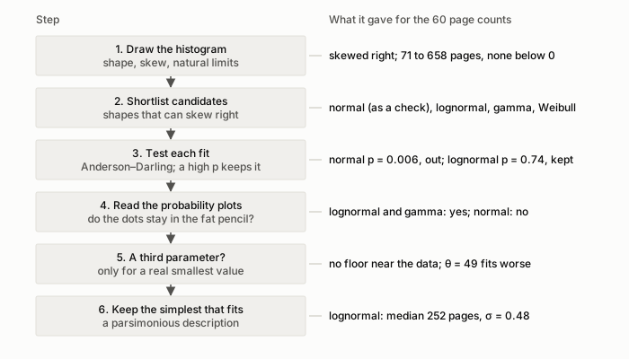 Figure 13.4. The decision path with the page counts’ result at each step, ending with a lognormal of median 252 pages and σ = 0.48.
From my notes. A comment by whuber on Cross Validated, saved in my notes: “It is impossible to have enough power to rule out a mixture.” The same comment explains that, without a theory to suggest a form, we fit a parametric distribution to get a parsimonious, approximate description of the data.
A mixture blends distributions, such as paperbacks and hardbacks with different typical lengths. A tiny share of one kind, or two nearly identical kinds, can escape any test, and mixtures need many parameters, so aim for a short, honest description, not the one true distribution.
Watch, read, try
- How to Identify the Distribution of Your Data — Jim Frost’s article that my notes kept.
- How to determine which distribution fits my data best? — COOLSerdash’s answer, with whuber’s comment.
- How to interpret a QQ plot? — Glen_b on reading Q–Q plots.
Check yourself. 1. An Anderson–Darling test gives p = 0.006 for a normal fit. What do you conclude, and why is a high p-value the hopeful result in this kind of test? 2. In a probability plot, the dots sit above the line at both ends and below it in the middle. Which way are the data skewed? 3. When is a three-parameter distribution with a threshold justified?
Answers. 1. Reject the normal at the 5% level. The null hypothesis of a fit test is that the distribution fits, so a high p-value means the data are compatible with it and the candidate stays. 2. To the right: both the smallest and the largest values are larger than the model expects, so the low tail is short and the high tail long. 3. When subject knowledge says there is a real smallest value, and the LRT P shows that the third parameter improves the fit.
14. Features: telling categories from numbers, and scaling
In one breath. Before a model can learn from a table, each column must be read as a quantity or a label, and quantities usually need rescaling so that none drowns out the others. Getting this wrong wastes training time at best and teaches the model nonsense at worst.
A feature is one column a model learns from, such as a book’s price; feature engineering turns raw columns into useful features, starting with one question: what kind of thing is this column?
Numbers that are really labels
A categorical column holds labels that sort things into groups, a numerical column quantities, and both can be stored as digits. The test is the one in Figure 14.1: does adding two values mean something?
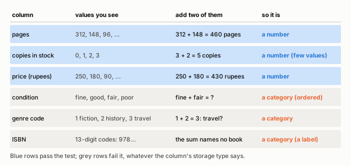 Figure 14.1. The addition test. Pages, copies in stock and price add up to meaningful totals (312 + 148 = 460 pages); condition, genre code and ISBN do not, so they are categories whatever their storage type.
Three copies and two make five, so copies in stock is a number although it takes only the values 0 to 3. Fiction (1) plus history (2) is not travel (3), so genre code is a category, and an ISBN is a label written in digits. Condition, from fine to poor, is an ordered category: fine beats fair, but fine plus fair means nothing. The pandas function select_dtypes picks columns by storage type but cannot know that genre code 2 is a label, so the call is yours. Chapter 25 shows how to encode categories, and a bar chart of the counts per category is the quickest way to look at them.
Why rescale at all
Page counts vary by about 130 pages across our books, the ages of eight books on a shelf by about 12 years. Gradient descent, which nudges each weight downhill on the error surface (chapter 8), suffers from such a mismatch: the surface becomes a long, narrow valley instead of a round bowl. Figure 14.4, at the chapter’s end, draws both to scale for a two-weight bowl whose curvatures are the two columns’ variances, a stylised error surface rather than a fitted regression. With raw pages and ages that bowl curves 112 times more sharply across the valley than along it. Gradient descent bounces between the walls and needs 257 steps to get within 1% of the bottom, even at its best fixed step size. Standardise both columns and one step suffices, the point of Andrew Ng’s lecture on normalising inputs.
Three ways to rescale, and the trouble with outliers
Min–max scaling maps the smallest value to 0 and the largest to 1. Standardisation, or the z-score, subtracts the mean and divides by the standard deviation. Robust scaling subtracts the median and divides by the interquartile range (IQR), the distance between the 25th and 75th percentiles. All three are straight-line rescalings that keep a distribution’s shape. Figure 14.2 applies them to eight book ages, 1, 2, 2, 3, 4, 5, 6 and 40 years, where 40 is an outlier, a value far from the rest.
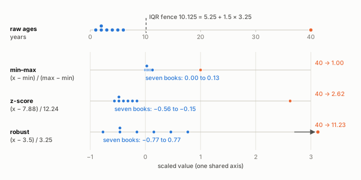 Figure 14.2. One outlier under three scalers. Min–max crowds the seven ordinary books into 0 to 0.13 and z-scores into −0.56 to −0.15; robust scaling spreads them from −0.77 to 0.77 and leaves the outlier far out at 11.23.
Min–max crowds the seven ordinary books into the bottom eighth of the range, and the z-score does little better, since the outlier drags the mean to 7.9 and the standard deviation to 12.2. Robust scaling uses the median (3.5) and IQR (3.25), which the outlier barely moves, so the ordinary books keep a spread of about 1.5 and the outlier stands out at 11.23. A comparison table in my notes said standardisation changes a distribution’s shape and resists outliers; Figure 14.2 shows it does neither.
Finding outliers, and squeezing large numbers
The IQR rule flags values more than 1.5 IQRs beyond the quartiles. With the upper quartile at 5.25, the fence is 5.25 + 1.5 × 3.25 = 10.125, which catches the 40-year-old book. The popular three-standard-deviation rule misses it, with a fence at 44.6, because the outlier inflates the mean and spread that judge it. Across several columns, the local outlier factor flags rows in much emptier space than their neighbours (20 by default in scikit-learn). Before deleting an outlier, ask whether it is a mistake: a 40-year-old book may be the shop’s most valuable copy.
Columns spanning orders of magnitude, such as copies printed, call for a logarithm. In Figure 14.3, four of six print runs between 800 and 2,000,000 crowd into one corner of an ordinary axis. After taking base-10 logarithms, each factor of ten is one equal step: as a Data Science Stack Exchange answer puts it, 10,000 − 1,000 becomes 4 − 3.
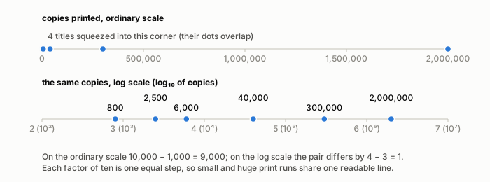 Figure 14.3. The log squeeze. Print runs from 800 to 2,000,000 crowd together on an ordinary axis and spread out on a log axis, where 10,000 − 1,000 = 9,000 becomes 4 − 3 = 1.
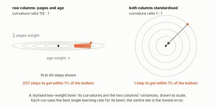 Figure 14.4. Why rescaling speeds up learning. In a stylised two-weight bowl whose curvatures are the two columns’ variances, raw pages and ages make it curve 112 times more sharply one way than the other and gradient descent needs 257 steps; after standardising both columns it needs 1.
A last trap hides in the target. If 5% of a catalogue are rare editions, a model that always answers “not rare” is right 95% of the time and useless. With such imbalanced classes, judge by precision and recall, not accuracy, and consider resampling.
From my notes. Numeric columns can be categorical. Domain knowledge tells them apart: total_coins can take few values but adding two of them makes sense; cabin_class (high, low, medium) makes no sense to add.
That is Figure 14.1’s addition test, with one refinement: cabin class, like a book’s condition, is an ordered category, whose order a model may use.
Watch, read, try
- Separate numerical and categorical variables — an answer using select_dtypes.
- pandas.DataFrame.select_dtypes — the pandas reference.
- Plotting categorical data with pandas and matplotlib — category counts drawn as bars.
- Feature Scaling — a Kaggle notebook on scalers.
- Scaling and Normalization — Alexis Cook’s Kaggle lesson.
- Compare different scalers on data with outliers — a Kaggle comparison of scalers.
- Compare the effect of different scalers on data with outliers — scikit-learn’s own comparison.
- Feature Engineering Tutorial — a Kaggle tutorial.
- Why take the log of some continuous variables? — the answer behind Figure 14.3.
- How to Remove Outliers for Machine Learning — Jason Brownlee on outlier rules.
- LocalOutlierFactor — the scikit-learn reference.
- Tips for Handling Imbalanced Data in Machine Learning — metrics and resampling for rare classes.
- Normalizing Inputs (C2W1L09) — Andrew Ng’s lecture behind Figure 14.4.
- Practical Deep Learning for Coders 2022, Lesson 3 — Jeremy Howard’s fast.ai lesson, at my saved point.
Check yourself. 1. A column holds shelf numbers from 1 to 12. Is it numerical or categorical? 2. Which of min–max scaling, standardisation and robust scaling changes the shape of a column’s distribution? 3. Why does the three-standard-deviation rule miss the 40-year-old book when the IQR rule catches it?
Answers. 1. Categorical: shelf 3 plus shelf 4 is not shelf 7 in any useful sense, so the numbers are labels. 2. None of them; all three are straight-line rescalings that keep the shape. 3. The outlier itself inflates the mean and the standard deviation, pushing the three-sd fence out to 44.6, while the quartiles, and so the IQR fence of 10.125, barely move.
15. Quantile normalisation
In one breath. Quantile normalisation forces several samples to share one distribution by giving the smallest value of every sample the same number, the second smallest the same number, and so on. It removes differences of scale between samples, which helps when those differences are technical and destroys information when they are real.
Three reviewers score the same five books for the shop’s newsletter. The first reviewer uses the whole scale from 1 to 5, the second is similar, and the third is generous, handing out scores up to 8. If you want to compare books across reviewers, the difference in generosity gets in the way. It is a difference in how each reviewer uses the scale, not in which books they liked.
A quantile, from chapter 12, is the value below which a given fraction of a sample falls. Quantile normalisation makes every sample have the same quantiles, and it does so in four steps, drawn in Figure 15.1. In the language of the method, each reviewer is a sample and each book is a feature.
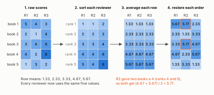 Figure 15.1. Quantile normalisation in four steps. The rank means are 1.33, 2.33, 3.33, 4.67 and 5.67; reviewer 2’s tied scores of 4 both become (4.67 + 5.67) / 2 = 5.17.
First, sort each reviewer’s scores from lowest to highest. Second, average across each rank: the three lowest scores are 1, 1 and 2, with mean 1.33, and the three highest are 5, 4 and 8, with mean 5.67. Third, give every reviewer that shared list of five means. Fourth, put the means back in each reviewer’s original order, so the book a reviewer liked most receives the largest mean. After the fourth step every reviewer uses the same five values, and only the order of the books differs. Ties need a rule. Reviewer 2 gave two books a 4, which occupy ranks 4 and 5, and the usual rule gives both the average of the two rank means, 5.17.
Where it came from, and what it assumes
The method comes from gene-expression microarrays, where each array (a sample) measures thousands of genes (the features) and arrays differ in brightness for purely technical reasons. In 2003 Ben Bolstad and colleagues compared ways of normalising such arrays and recommended the quantile method, which did well both in speed and on their measures of bias and variance. The whole method rests on one assumption: that the samples really should have the same distribution. For microarrays that means only a small share of the genes change between conditions. When the assumption holds, the differences that quantile normalisation removes are technical noise. When it fails, the differences it removes are the answer you were looking for.
A real difference, erased
Figure 15.2 shows the failure on a small scale. Two critics and two fans score five books. The fans genuinely score books 1 to 4 three points higher than the critics do, and both groups score book 5 the same. Within each group, one reviewer marks a point lower than the other, which is the kind of technical difference quantile normalisation is meant to remove.
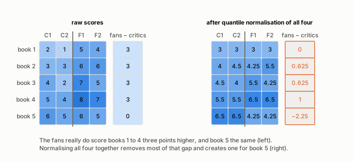 Figure 15.2. Normalising all four columns together. The real gap of 3 points shrinks to 0, 0.625, 0.625 and 1, and book 5, which both groups scored equally, gains a false gap of −2.25.
After normalising all four columns together, the real gap of 3 points nearly vanishes, and book 5 now appears to be disliked by the fans, with a gap of −2.25 that exists only in the processed numbers. Forcing the fans’ generous scores onto the same five values as the critics’ scores has pushed the fans’ book 5 down the ranking.
Normalising within each class
The repair is to normalise each group separately. Zhao, Wong and Goh (2020) call this class-specific quantile normalisation: split the data by class first, normalise each part, then put them back together. Figure 15.3 applies it to the critics and the fans.
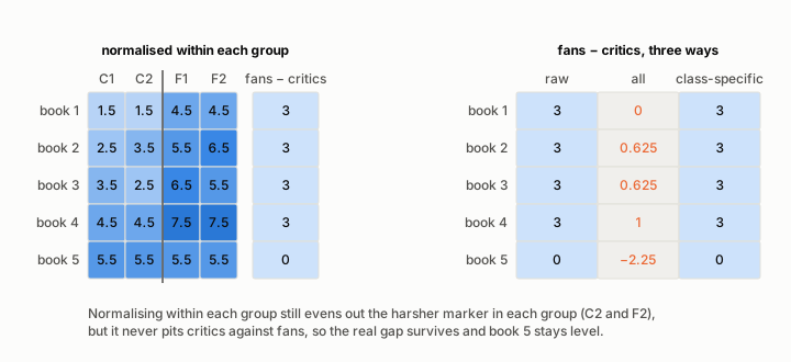 Figure 15.3. Class-specific normalisation. Each group’s harsher marker is evened out, and the gaps return to the true 3, 3, 3, 3 and 0, where normalising everything had given 0, 0.625, 0.625, 1 and −2.25.
Within each group the harsher marker is evened out, the two critics now share one set of values and the two fans another, and the real gap between the groups survives untouched. Zhao and colleagues compare five variants: All (the plain method on everything), Class-specific, Discrete (split by class and by batch), Ratio, and qsmooth, which weighs the differences between groups against the variation within them. Their advice is that if quantile normalisation must be used, the class-specific variant is the one to choose. Hicks and Irizarry (2014) proposed a statistical test, called quantro, for checking whether the assumption of equal distributions is safe before normalising at all.
My notes placed a different technique under the same heading, so it is worth separating the two. scikit-learn’s QuantileTransformer works on one feature at a time: it maps a column’s values onto a uniform or a normal distribution through their ranks. That spreads out the most common values, tames outliers, and can distort the correlations between columns. Quantile normalisation in the sense of this chapter works across samples and makes them share one distribution built from their own values. Both use ranks, but they answer different questions.
From my notes. The best article on quantile normalisation is Zhao, Wong and Goh (2020). I copied its warning that after normalisation the profiles “look deceptively similar, even if the underlying classes are in fact, very different” (Zhao, Wong and Goh), and that the method can wipe out true signals and create false ones.
Figure 15.2 is that warning in miniature. After normalisation every sample looks tidy by construction, and a perfect-looking result is a reason to ask what was removed, not a reason to relax.
Watch, read, try
- How to do quantile normalization correctly for gene expression data analyses — Zhao, Wong and Goh (2020), the open-access article behind this chapter.
- Quantile Normalization, Clearly Explained!!! — StatQuest’s explanation of the method.
- Quantiles and Percentiles, Clearly Explained!!! — StatQuest on the quantiles the method is named after.
- Mastering Quantile Normalization in R: A Step-by-Step Guide — an R-bloggers walk-through with code.
- When to use Quantile Normalization? — Hicks and Irizarry on the assumption, and the quantro test for it.
- Non-linear transformation in scikit-learn — the scikit-learn guide to QuantileTransformer, the per-feature cousin.
Check yourself. 1. After quantile normalisation, what do all the samples have in common, and what can still differ between them? 2. Why did book 5 gain a false gap in Figure 15.2? 3. When is plain quantile normalisation over all samples safe?
Answers. 1. They share exactly the same set of values, the rank means; only the order of the features within each sample differs. 2. The fans’ other scores were higher, so book 5’s unchanged score ranked lower among the fans than among the critics, and after normalisation that lower rank became a lower value. 3. When the samples really should share one distribution, so that the differences removed are technical, for example when only a small share of features differ between groups.
16. Batch normalisation
In one breath. Batch normalisation standardises each unit’s weighted sums across the examples of a mini-batch, then lets the network rescale them with two learned numbers. It made deep networks much faster to train, although the reason it works is still debated.
Chapter 14 rescaled the inputs so that the error bowl became round and gradient descent could take long, confident steps. Inside a network the same problem returns at every layer. The weighted sums that one layer passes to the next change their scale and centre as training changes the weights, and, as Ioffe and Szegedy saw it, later layers keep chasing a moving target. In 2015 Sergey Ioffe and Christian Szegedy proposed normalising those sums as part of the network itself.
A mini-batch is the small group of training examples used for one step of gradient descent, for instance six books out of the whole catalogue. A unit is one neuron of a layer, which computes a weighted sum of its inputs before its activation function (chapter 7 builds one).
Where it sits
Figure 16.1 shows the place of the new step. A unit first computes its weighted sum z of the inputs; batch normalisation turns z into a standardised value and then into its own output; the activation, here ReLU, comes last. The unit’s usual bias can be dropped, because the shift β introduced below plays the same part.
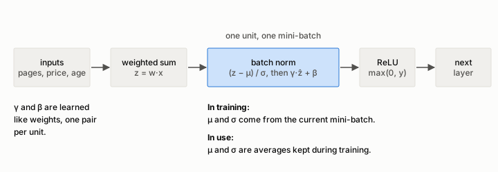 Figure 16.1. Batch normalisation sits between a unit’s weighted sum and its activation. In training it uses the mini-batch’s mean and standard deviation; in use it uses averages kept during training.
Four lines of arithmetic
Suppose one unit produces these weighted sums for a mini-batch of six books: 14, 9.5, 21, 12.5, 17 and 10. Ioffe and Szegedy’s algorithm has four lines.
- Take the mean of the batch: 14.
- Take the variance of the batch, the average squared distance from the mean: 16.083, so the standard deviation is 4.01.
- Normalise: subtract the mean and divide by the standard deviation. The six values become 0, −1.12, 1.75, −0.37, 0.75 and −1.00. A tiny constant ε is added to the variance first so that a batch of identical values cannot cause a division by zero.
- Scale and shift: multiply by a learned number γ and add a learned number β.
Figure 16.2 follows the six values through the steps, with γ = 2 and β = 1 standing in for values the network might learn.
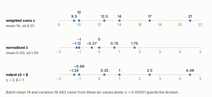 Figure 16.2. One unit’s weighted sums for six books. The batch mean 14 and standard deviation 4.01 turn them into values with mean 0 and sd 1; γ = 2 and β = 1 then give −1.24, −0.99, 0.25, 1, 2.5 and 4.49.
Why undo the normalisation with γ and β? Forcing every unit to mean 0 and standard deviation 1 would limit what the layer can express. Ioffe and Szegedy’s example is the sigmoid activation: inputs held near 0 stay in the sigmoid’s nearly straight middle section, so the unit could only act almost linearly. With γ and β learned like any other weight, the network can choose any centre and spread it likes, including, if that turns out best, the original ones: setting γ to the batch’s standard deviation and β to its mean gives back the raw sums.
In the convolutional networks of Part IV, one filter produces a whole map of values, one per position of the image. There, batch normalisation pools the statistics over every example in the mini-batch and every position in the map, so all positions are treated alike, and it learns one γ and one β per map. A mini-batch of 32 book covers with 6 × 6 maps gives 32 × 36 = 1,152 values for each mean and variance.
Training and use
During training the mean and variance come from the current mini-batch, so each example’s output depends a little on which other books share its batch. Once training is over, a single book may arrive on its own, and a batch of one has no useful spread. So the network keeps running averages of the batch statistics during training and uses those fixed numbers afterwards. Ioffe and Szegedy estimate the variance for this purpose with a small correction, multiplying by m/(m − 1) for batches of m examples; for our batch of six that turns 16.083 into 19.3.
The results were striking. On ImageNet, the image-classification benchmark whose yearly challenge had about 1.2 million labelled training photos in 1,000 classes, their batch-normalised network matched the accuracy of the Inception network it was built on with 14 times fewer training steps, and an ensemble of such networks reached a top-5 error of 4.9% on the validation images. Batch normalisation also allows much larger learning rates and makes training less sensitive to the starting weights.
Why it works is less settled. Ioffe and Szegedy explained it as a cure for internal covariate shift, their name for the drifting distribution of each layer’s inputs. In 2018 Santurkar and colleagues tested that explanation and found that the method’s success has little to do with such drift; instead, batch normalisation makes the error surface smoother, so gradients are more reliable and larger steps are safe. The four lines of arithmetic are not in dispute; the story told about them is.
Watch, read, try
- Normalizing Activations in a Network (C2W3L04) — Andrew Ng’s lecture introducing batch normalisation.
Check yourself. 1. Which numbers does batch normalisation learn, and which does it compute from the data? 2. Why can the unit’s own bias be dropped? 3. What replaces the mini-batch statistics when the trained network scores a single book?
Answers. 1. It learns γ and β for each unit; it computes the mean and variance from each mini-batch during training. 2. Subtracting the batch mean removes any constant added before it, and β supplies a learned shift after it. 3. Running averages of the mean and variance collected during training.
Part IV: Seeing: convolutional networks
17. Images as numbers, and the convolution operation
In one breath. A digital image is a grid of numbers, one grid for a grey picture and three for a colour one, and a convolution slides a small grid of weights across it, multiplying and adding at every stop. That single operation, repeated with learned weights, is how a network learns to read pictures.
Photograph the covers of the books in the shop and each photo becomes a table of numbers. One cell of the table is a pixel, and its number says how bright that spot is. To keep the arithmetic in this part small, our covers use brightness from 0 (dark) to 9 (bright); a real image file stores 0 to 255. Figure 17.1 shows the cover used throughout Part IV: six pixels by six, dark except for a bright hollow square.
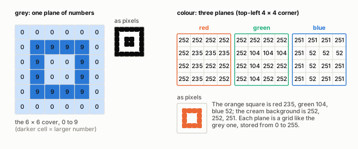 Figure 17.1. An image is numbers. The grey cover is one 6 × 6 plane of 0s and 9s; the colour version stores three planes, and its orange square is red 235, green 104, blue 52 in every pixel.
A colour photo stores three numbers per pixel, one each for red, green and blue light, so it is three grids stacked on top of each other. Each grid is a channel. The orange square of our colour cover is red 235, green 104 and blue 52 at every one of its pixels, and the cream background is 252, 252 and 251. A grey image has one channel, a colour image three, and inside a network the count of channels grows much larger.
The convolution operation
A kernel is a small grid of weights, here three by three. The kernel of this chapter has 1s in its corners and centre and 0s elsewhere. To apply it, lay it over the top-left three-by-three window of the cover, multiply each weight by the pixel beneath it, and add the nine products. The total is one number of the output. Then slide the kernel one pixel to the right and repeat, row after row. Figure 17.2 follows the first six positions.
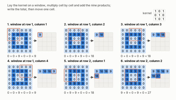 Figure 17.2. The kernel slides one cell at a time. The first window gives 0 + 0 + 9 + 0 + 0 = 9, the next 18, and the window at row 2, column 2 gives 27, where three of the kernel’s five 1s land on the bright frame.
The finished output is a four-by-four grid, 9, 18, 18, 9 along its top row and 27 at its four middle cells. It is called a feature map, because it shows where in the image the kernel’s pattern appears. Mathematicians define convolution with the kernel flipped before it slides; deep-learning libraries skip the flip and still call the operation convolution, as Goodfellow, Bengio and Courville note in their textbook. For a kernel that is learned, the difference does not matter, and ours is symmetric anyway. Chapter 24 returns to the flip.
Padding
The output is smaller than the input, six by six in and four by four out, because a three-by-three window fits only four times across six pixels. The pixels on the border also never sit at the centre of a window. Padding fixes both: add a ring of zeros around the image before sliding. With one ring, the output of a three-by-three kernel is the same size as the input (Figure 17.3). The corner output now comes from a window that is mostly padding, 0 + 0 + 0 + 0 + 9 = 9.
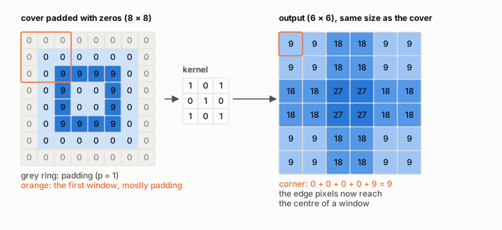 Figure 17.3. Zero padding of one cell. The output is 6 × 6, the same size as the cover, and the corner window, mostly padding, gives 9.
Stride
The stride is how far the kernel moves between positions. With a stride of 2 it jumps two pixels at a time, and the output shrinks to two by two: 9, 18, 18 and 27 (Figure 17.4, left). Only two windows fit across, and the cover’s last row and last column are never read. With padding of 1 and stride 2 the output is three by three, and now the last row and column of the padded image are skipped; Dumoulin and Visin draw exactly this case, a six-pixel input with padding 1 and stride 2, in their guide to convolution arithmetic. A stride of 2 gives the same numbers as computing every window and keeping every second one.
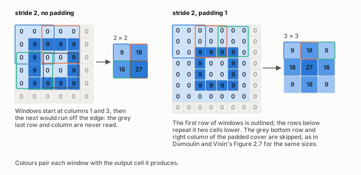 Figure 17.4. Stride 2. Without padding the output is 2 × 2 and the last row and column go unread; with padding 1 it is 3 × 3 and the padded border’s last row and column are skipped.
One formula for every size
All these sizes follow from one rule (Dumoulin and Visin, Relationship 6). For an input of i pixels, a kernel of k, padding of p and a stride of s, the output has
\[o = \left\lfloor \frac{i + 2p - k}{s} \right\rfloor + 1\]pixels, where the brackets round down. Figure 17.5 works it for eight settings on our six-pixel cover.
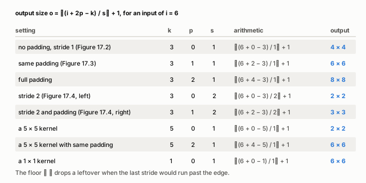 Figure 17.5. Output sizes for a 6 × 6 input. No padding gives 4 × 4, same padding 6 × 6, full padding 8 × 8, and stride 2 gives 2 × 2, or 3 × 3 with padding.
These operations became famous in 2012, when a convolutional network later known as AlexNet won the ImageNet challenge. Its top-5 error, the share of test images whose correct label was missing from the model’s five best guesses, was 15.3%, against 26.2% for the second-best entry. It had 60 million parameters, 650,000 neurons and five convolutional layers (Krizhevsky, Sutskever and Hinton, 2012).
From my notes. My CNN note opens with a sentence I copied in bold from an Analytics Vidhya introduction to convolutional networks. In my own words: the convolutional layers reduce an image to something a classifier can use, without dropping the features that decide the answer.
That is a fair summary of the whole of Part IV, which shows how the reduction is done: kernels pick out features (chapter 18), shared weights keep the cost low (chapter 19), and pooling and strides shrink the grid (chapter 20).
Watch, read, try
- A guide to convolution arithmetic for deep learning — Dumoulin and Visin’s guide, the source of the formula and of the padding and stride cases above.
- conv_arithmetic — the animations that accompany the guide, one per case.
- Convolution demo — the CS231n course’s interactive convolution demo.
- CNN Explainer — an interactive visualisation of a convolutional network.
- Animated AI — a collection of animations about neural-network operations.
- Convolution Demo — deeplizard’s interactive convolution.
- Convolutions in Deep Learning - Interactive Demo App — deeplizard’s video on the same demo.
- But what is a neural network? — the first chapter of 3Blue1Brown’s series on neural networks.
- CNN: Convolutional Neural Networks Explained - Computerphile — Computerphile’s introduction to convolutional networks.
- Neural Networks Part 8: Image Classification with Convolutional Neural Networks — StatQuest on image classification with convolutional networks.
- ImageNet Classification with Deep Convolutional Neural Networks — the 2012 AlexNet paper.
Check yourself. 1. A 6 × 6 image, a 3 × 3 kernel, no padding and stride 1: what size is the output? 2. What padding keeps the output of a 5 × 5 kernel the same size as its input at stride 1? 3. In a stride-2 pass over the 6 × 6 cover without padding, which pixels are never read?
Answers. 1. 4 × 4, since ⌊(6 + 0 − 3) / 1⌋ + 1 = 4. 2. Two rings of zeros, p = 2, since ⌊(i + 4 − 5) / 1⌋ + 1 = i. 3. The last row and the last column, because windows start at the first and third pixels and a third window would run off the edge.
18. Kernels, filters, channels and bias
In one breath. With a colour image a filter is not one kernel but a stack of them, one per input channel, whose results are added together with a single bias to make one output channel. A layer with N filters therefore turns its input into N channels, and the words kernel, filter and channel stop meaning the same thing.
With a grey image there is only one channel, and the three-by-three kernel of chapter 17 is the whole story. The words kernel and filter then mean the same thing, and many tutorials use them that way. The difference appears as soon as the input has more than one channel.
One filter, three kernels
A filter for a colour image holds one kernel for each input channel: a three-by-three kernel for red, another for green, another for blue, three by three by three in all. Each kernel slides over its own channel and produces its own map, and the three maps are added cell by cell into one. Dumoulin and Visin describe it this way, and the squeeze-and-excitation paper of chapter 23 writes the same sum as its first equation.
Figure 18.1 works it on a small four-by-four corner of a cover, with small numbers in each channel. The red kernel subtracts the right column of each window from the left; the green kernel compares each pixel with its four neighbours; the blue kernel subtracts the bottom row from the top. Their maps are [0, −1; 2, 3], [−2, 2; 5, 4] and [1, 0; 0, −2], and their sum is [−1, 1; 7, 5].
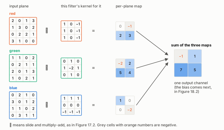 Figure 18.1. One filter, three kernels. Each colour plane is convolved with its own kernel, and the three 2 × 2 maps add up to −1, 1, 7 and 5.
Because each channel has its own kernel, a filter can weigh the channels differently. A filter whose red kernel has large weights and whose other kernels are nearly zero responds mostly to patterns in red. Adding the channels together is also what lets a filter respond to a colour rather than to one plane. The orange square of chapter 17 is strong in red and weak in blue, so a filter with a positive red kernel and a negative blue kernel responds to orange areas far more than to cream ones, where red and blue are nearly equal. No single channel could tell those two apart by itself.
One bias per filter
After the sum comes the bias: a single number that belongs to the filter and is added to every cell of its map. With a bias of −2, the map [−1, 1; 7, 5] becomes [−3, −1; 5, 3], and the ReLU activation of chapter 7 then turns the negative cells into zeros, leaving [0, 0; 5, 3] (Figure 18.2). The bias sets how strong the evidence must be before the filter reports anything.
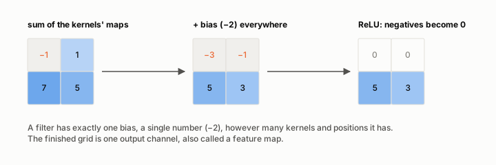 Figure 18.2. The filter’s single bias, −2, is added to every cell, and ReLU then zeroes the negatives: the output channel is 0, 0, 5 and 3.
Many filters, many channels
A layer usually has many filters, each with its own kernels and bias, and each produces one output channel. Four filters on a three-channel input give four output maps, stacked into a new block with four channels (Figure 18.3). The next layer then needs four kernels in each of its filters, one for each of these channels. The parameter count follows directly: four filters of 3 × 3 × 3 weights plus one bias each make 4 × 28 = 112. The CS231n course notes give a larger example: 96 filters of 11 × 11 × 3 on a colour image make 96 × 364 = 34,944 parameters.
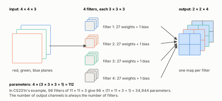 Figure 18.3. Four filters, four output channels. Each filter spans all three input channels; the layer has 4 × (3 × 3 × 3 + 1) = 112 parameters.
The words that caused the confusion can now be pinned down.
| word | what it is | in Figure 18.1 |
|---|---|---|
| kernel | a small grid of weights for one input channel | each 3 × 3 grid |
| filter | one kernel per input channel, plus one bias; makes one output channel | the three kernels and the bias together |
| channel | one plane of a layer’s input or output | the red, green and blue planes; the summed map |
| feature map | an output channel, showing where the filter’s pattern appears | the 2 × 2 result |
| feature detector | an informal name for a filter, after what it does | the whole filter |
| receptive field | the region of the original image that can change one output number | here 3 × 3 pixels in each channel; larger in deeper layers |
From my notes. Kernel, feature detector, filter (collection of kernels), receptive field: all are the same.
The note has the right instinct for a grey image, where one kernel is the whole filter and “feature detector” is only a nickname for it. With several channels the words part company: a filter is the collection of kernels, one per channel, as the note’s own brackets say. The receptive field is a different kind of thing, an area of the image rather than a set of weights. It equals the kernel’s size only in the first layer, and chapter 21 shows how it grows after that.
From my notes. From the CS231n notes: with a 5 × 5 filter on a colour image, each unit of the layer has weights to a 5 × 5 × 3 block of the input.
That example is exact: the kernels always run the full depth of their input, so a 5 × 5 filter on a three-channel image holds 5 × 5 × 3 = 75 weights, plus one bias. The notes call the 5 × 5 size the receptive field, which is right for this first layer only.
Watch, read, try
- Convolutional Neural Networks (CS231n) — the Stanford course notes behind the 75-weight and 34,944-parameter examples.
- Conv Nets: A Modular Perspective — Chris Olah on convolutional layers as reusable blocks.
Check yourself. 1. A layer receives 16 channels and has 32 filters of size 3 × 3. How many kernels, weights and biases does it have? 2. How many channels does it output? 3. Why is the bias added once to the summed map rather than once to each channel’s map?
Answers. 1. 32 × 16 = 512 kernels, 512 × 9 = 4,608 weights and 32 biases. 2. 32, one per filter. 3. A filter has exactly one bias; separate biases on each channel’s map would only add up to one number anyway.
19. Why convolution works
In one breath. A convolution is an ordinary linear layer with most of its weights forced to zero and the rest shared, which makes it tiny compared with a dense layer and builds in the belief that nearby pixels belong together. That belief is right for pictures, and it is why convolutional networks learn from images so much more efficiently than dense networks do.
A linear layer in disguise
Take a four-by-four input and a three-by-three kernel, which give a two-by-two output. Read the 16 input pixels row by row into a list and the 4 outputs likewise. A dense layer, in which every output is a weighted sum of every input, would need a 4 × 16 matrix of 64 independent weights. The convolution is also a weighted sum of the inputs, so it too has a 4 × 16 matrix, but a very particular one: each row holds the kernel’s nine weights at the positions of that output’s window and zeros everywhere else, and every row repeats the same nine weights, shifted (Figure 19.1). Dumoulin and Visin write out this matrix in their guide.
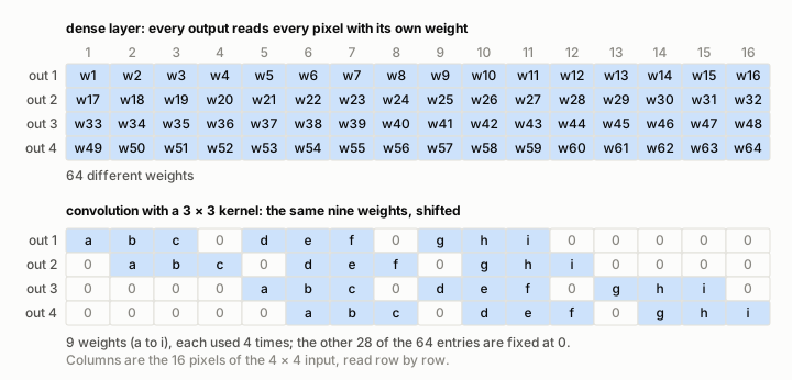 Figure 19.1. The same mapping as a dense layer and as a convolution. The dense layer has 64 free weights; the convolution uses 9, each in four places, and fixes the other 28 entries at 0.
Two ideas make the difference, and Goodfellow, Bengio and Courville name them sparse interactions, each output depending on a few inputs, and parameter sharing, the same weights used at every position. At the scale of real photos the saving is dramatic. A 224 × 224 colour photo holds 150,528 numbers. A dense layer from it to only 1,000 hidden units needs 150,528,000 weights, while a layer of 64 three-by-three filters needs 1,728 weights and 64 biases (Figure 19.3, right).
Locality, the belief built in
Fixing most weights at zero and sharing the rest is a strong assumption, which the same textbook calls an infinitely strong prior: whatever the layer learns, it can only combine nearby pixels, and it must treat every position alike. For pictures that assumption is sound. A pixel is usually similar to its neighbours, and an edge or a corner means the same thing wherever it appears. For the shop’s inventory spreadsheet it would be nonsense. Its columns (pages, price, age, genre) could be listed in any order, and a kernel sliding across neighbouring columns would look for shared patterns that are not there. Convolutions suit data laid out on a grid whose neighbours are related, such as images, or sound laid out in time.
An edge detector by hand
Before networks learned their own kernels, people designed them. The Sobel kernel, presented by Irwin Sobel and Gary Feldman at the Stanford Artificial Intelligence Laboratory in 1968, is [1, 0, −1; 2, 0, −2; 1, 0, −1]. On each window it subtracts the right-hand column from the left-hand one, counting the middle row twice. Figure 19.2 applies it to an eight-by-eight image with a bright four-by-four block. Flat areas give 0, and so does the inside of the block. Along the block’s left edge, where brightness jumps from 1 to 9, the output is −8, −24 and −32; along its right edge it is +8, +24 and +32. The top and bottom edges give 0, because the kernel only measures change from left to right.
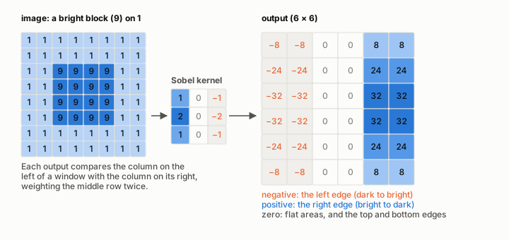 Figure 19.2. A hand-made edge detector. The Sobel output is 0 on flat regions, −8 to −32 along the block’s left edge and +8 to +32 along its right edge.
Because this kernel measures change in the horizontal direction, it lights up edges that run vertically. That is why the article in my notes calls it a vertical edge detector in its text and labels it a horizontal Sobel kernel in its figure: both names describe the same kernel, one by what it finds and one by what it measures. Figure 19.3 makes the locality visible: each output number comes from one small patch of the image.
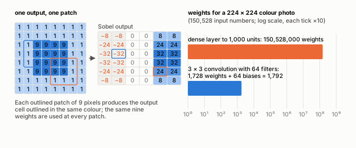 Figure 19.3. Each output sees one patch, which is why so few weights suffice. For a 224 × 224 colour photo, a dense layer to 1,000 units needs 150,528,000 weights; 64 convolution filters need 1,792 parameters.
Learning the kernels instead
Deep learning keeps the sliding and lets gradient descent choose the weights. The first layers of trained networks end up with kernels much like the hand-made ones. AlexNet’s first layer learned 96 kernels of 11 × 11 × 3 that the authors describe as frequency- and orientation-selective, plus coloured blobs (Krizhevsky and colleagues, Figure 3). Chris Olah, Alexander Mordvintsev and Ludwig Schubert show what deeper units respond to with feature visualisation: start from random noise and adjust the picture, step by step, until one chosen unit responds as strongly as possible. The output of a convolution is itself a grid, still shaped like an image, so another convolution can run on top of it, and chapter 21 follows what that stacking achieves.
Kernels learned on one large collection of photos are useful on others. François Chollet’s Keras post of 2016, built on 1,000 photos each of cats and dogs, reached about 80% accuracy with a small network trained from scratch, about 90% by reusing the convolutional layers of a network trained on ImageNet, and 94% by also fine-tuning the top layers of that network.
From my notes. Convolution layers do what they do best, extracting features from data with two spatial dimensions; the extracted features are then passed to linear layers, which are great at finding relationships between feature vectors and targets.
That is the classic design. AlexNet ends its five convolutional layers with three fully connected layers and a softmax, the function that turns the last layer’s scores into probabilities that add up to one. GoogLeNet ends with one linear layer after averaging each channel down to a single number.
Watch, read, try
- How Blurs & Filters Work - Computerphile — Computerphile on blurring and filtering images with kernels.
- How convolutional neural networks work, in depth — Brandon Rohrer’s long walk-through.
- MIT 6.S191 (2023): Convolutional Neural Networks — Alexander Amini’s lecture, saved next to the note above.
- Feature Visualization — Olah, Mordvintsev and Schubert on seeing what units respond to.
- Lucid — the open-source library behind those pictures.
- DeepVis Toolbox — Jason Yosinski’s toolbox for visualising a trained network.
- Deep Learning for Computer Vision (Andrej Karpathy) — the lecture through which my notes found the toolbox.
- Why use softmax as opposed to standard normalization? — a Stack Overflow discussion of the last step of a classifier.
- Building powerful image classification models using very little data — Chollet’s post on reusing trained convolutional layers.
Check yourself. 1. How many weights does a dense layer need to map a 6 × 6 image to a 4 × 4 output, and how many does a 3 × 3 convolution need? 2. Why would a convolution be a poor choice for a table of book prices, ages and genres? 3. On the Sobel output of Figure 19.2, why are the top and bottom edges of the block zero?
Answers. 1. 36 × 16 = 576 for the dense layer and 9 for the convolution. 2. The columns have no natural neighbours, so there is no local pattern to find and no reason to share weights across positions. 3. The kernel compares the left and right columns of each window; along a horizontal edge those columns are equal, so the difference is zero.
20. Pooling and strides
In one breath. Pooling shrinks a feature map by summarising each small window with one number, usually its largest, so that later layers handle fewer values and care less about exact positions. Many modern networks shrink with strided convolutions instead, but the trade of exact position for robustness remains.
A pooling layer slides a window over each channel, like a convolution, but instead of weights it applies a fixed rule. Max pooling keeps the largest number in the window; average pooling keeps the mean. With two-by-two windows and a stride of 2, the four-by-four grid of Figure 20.1 becomes two by two: max pooling gives 9, 5, 6 and 9, average pooling 5.25, 2.5, 3 and 5.5. Pooling has no weights to learn and works on each channel separately.
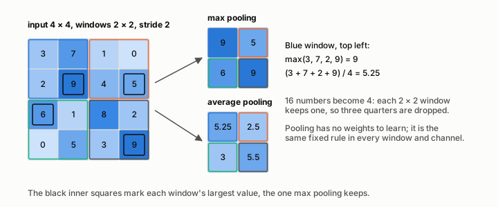 Figure 20.1. Pooling a 4 × 4 map with 2 × 2 windows and stride 2. Max pooling keeps 9, 5, 6 and 9; average pooling gives 5.25, 2.5, 3 and 5.5.
The output size follows the rule of chapter 17 without padding: ⌊(4 − 2) / 2⌋ + 1 = 2. A two-by-two pool with stride 2 keeps one value out of four, discarding three quarters of the activations, as the CS231n notes put it. They also report that max pooling has worked better in practice than average pooling, which used to be common. Averaging survives at the very end of many networks as global average pooling, which squeezes each whole channel into one number; Lin, Chen and Yan introduced it in 2013 as an easier-to-interpret replacement for the final fully connected layers.
Why shrink at all
Shrinking a map makes every later layer cheaper. A 224 × 224 map with 64 channels holds 3,211,264 numbers; after one 2 × 2 pool with stride 2 it holds 802,816, a quarter as many, and every later convolution has a quarter as many positions to visit. Shrinking also widens what the next layer sees, because each of its kernels now spans pixels that were twice as far apart (chapter 21 makes this exact). Max and average pooling summarise differently: the maximum reports whether a feature is present anywhere in the window, the average how much of it there is. During training, max pooling sends the error signal back only to the value it kept, which the CS231n notes describe as remembering where each maximum came from.
Equivariant and invariant
Two words describe how a layer reacts when its input shifts. A layer is equivariant to shifts when moving the input moves the output by the same amount, and invariant when moving the input leaves the output unchanged. Figure 20.2 shows both. A detector kernel of three 1s turns a bright bar into the response 9, 18, 27, 18, 9; shift the bar one cell and the whole response shifts one cell. Convolution is equivariant, which is what lets one detector find its pattern anywhere. For a network that sorts book covers, invariance is the useful half: whether the title block sits two pixels further left should not change the answer “cookbook”. Now take the maximum over each half of the response. The peak value 27 stays in the left half after the shift, so that pooled number does not change, but the right half changes from 9 to 18. Goodfellow, Bengio and Courville describe pooling as making a representation approximately invariant to small translations: most pooled values survive a small shift, and a larger shift can move the peak into another window.
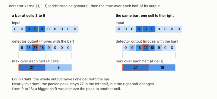 Figure 20.2. Shifting the bar one cell. The detector’s output moves one cell with it (equivariance); the pooled peak stays 27 in the left half (approximate invariance), while the right half changes from 9 to 18.
Strided convolutions instead of pooling
A convolution with stride 2 also halves the size of a map, and unlike pooling it learns how to summarise. In 2015 Springenberg and colleagues showed that max pooling can be replaced by a convolution with a larger stride without losing accuracy. ResNet, the network of chapter 23, shrinks its maps inside the network with stride-2 convolutions; it keeps one max-pooling layer right after its first convolution and a global average pool at the end (He and colleagues, Table 1). The CS231n notes add that dropping pooling has also mattered for networks that generate images, and that future designs may use very little pooling at all.
From my notes. Copied from Irhum Shafkat’s article: newer networks such as ResNet do without pooling inside the network and shrink their feature maps with strided convolutions instead.
The note is right about the inside of ResNet. The two exceptions are worth knowing: the single max pool after the first layer and the global average pool before the classifier.
Watch, read, try
- Translation Invariance & Equivariance in Convolutional Neural Networks — a Paperspace article on what pooling does to shifts.
- What is the difference between “equivariant to translation” and “invariant to translation” — Data Science Stack Exchange answers with a one-dimensional example like Figure 20.2.
- What are Pooling Layers in Deep Neural Networks? — a video introduction to pooling layers.
- Max Pooling Demo — deeplizard’s interactive max pooling.
- Pooling layers — Dremio’s glossary page on pooling.
Check yourself. 1. What do 2 × 2 max pooling and average pooling give for the window 2, 8, 5, 1? 2. Is a convolution equivariant or invariant to shifts? 3. Name one way to halve the size of a feature map without a pooling layer.
Answers. 1. Max pooling gives 8; average pooling gives 16 / 4 = 4. 2. Equivariant: shifting the input shifts its output. 3. A convolution with stride 2.
21. Receptive fields and the visual hierarchy
In one breath. The receptive field of a unit is the patch of the original image that can influence it, and it grows with every layer, fastest after strides and pooling. Growing fields let deep layers combine small patterns into large ones, from edges to whole objects.
The term comes from neuroscience. Sherrington used it in 1906 for an area of the body’s surface where a stimulus could trigger a reflex, and it was later extended to the region of the visual field where light makes a neuron respond. In the brain’s visual pathway these fields grow at each stage, from about half a degree to two degrees of the visual field near its centre in the primary visual cortex to around 30 degrees in a later area, the inferior temporal cortex (Alonso and Chen, Scholarpedia). Convolutional networks behave in the same way.
In a network, the receptive field of a unit is the set of input pixels that can change its value. In the first layer it is the kernel’s window. In the second layer each unit reads a window of first-layer units, each of which reads its own window of pixels, so the field widens.
How fast it grows
Figure 21.1 follows one unit down through three layers of three-wide kernels. With stride 1 everywhere, the unit sees 3 pixels after one layer, 5 after two and 7 after three. If the first layer has stride 2 instead, its units sit two pixels apart, each later kernel spans twice the distance, and the fields become 3, 7 and 11.
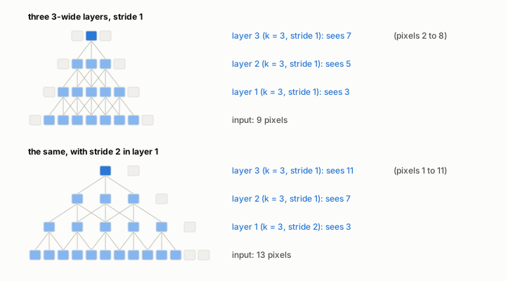 Figure 21.1. Receptive fields grow with depth. Three 3-wide layers with stride 1 see 3, 5 and 7 pixels; with stride 2 in the first layer they see 3, 7 and 11.
The general rule, from Araujo, Norris and Sim (2019), keeps two numbers as it walks up the layers: the field size r, and the jump j, the distance in input pixels between neighbouring units of the current layer. Start with r = 1 and j = 1. For each layer with kernel k and stride s, first widen the field, r becomes r + (k − 1) × j, then update the jump, j becomes j × s. Written out for L layers, that is
\[r = 1 + \sum_{l=1}^{L} (k_l - 1) \prod_{i=1}^{l-1} s_i\]For the stride-1 stack, r = 1 + 2 + 2 + 2 = 7; with stride 2 first, r = 1 + 2 + 4 + 4 = 11.
My notes kept a different formula from a Kaggle post, RF = (K − 1) × stride + 1, presented as the receptive field of a layer. It is one step of the rule above: the width covered by K taps whose inputs lie “stride” pixels apart. A three-wide kernel reading a layer whose units are two pixels apart covers (3 − 1) × 2 + 1 = 5 pixels, which is also the width of a three-tap kernel dilated by 2 (chapter 22). A single layer applied directly to an image always sees K pixels, whatever its own stride; its stride only widens the fields of the layers that come after it.
The centre counts most
Not every pixel in a receptive field matters equally. With all weights equal, the influence of a pixel on a unit is the number of paths from the pixel to the unit through the layers. Figure 21.2 counts them for three three-by-three layers: 1 path from each corner of the seven-by-seven field, 49 from its centre, and half of all 729 paths start in the middle three by three. Luo, Li, Urtasun and Zemel (2016) defined the effective receptive field, the part of the field that actually carries weight, and showed that it has a Gaussian shape that fills only a fraction of the full field.
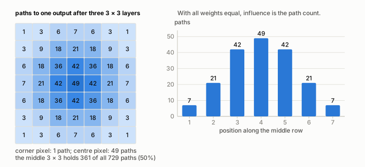 Figure 21.2. Paths from each pixel to one unit after three 3 × 3 layers. The corners have 1 path, the centre 49, and the middle 3 × 3 holds 361 of the 729 paths.
From my notes. A passage I saved in quotation marks next to a link to AI Summer’s article on receptive fields, an idea that article credits to Luo and colleagues: in the forward pass, pixels near the centre of a receptive field can pass their information to the output along many different paths, while pixels near its edge have very few; in the backward pass the gradient flows back along the same paths, so the centre pixels receive a much larger share of it.
Figure 21.2 is that passage in numbers. The same path counts that carry a centre pixel’s influence forward carry the error signal back to it during training.
From edges to objects
As fields grow, units can respond to larger and more complicated patterns. Goodfellow, Bengio and Courville illustrate the idea with images from Zeiler and Fergus (2014): early layers respond to edges, the next to corners and contours, the next to parts of objects, and the last to whole objects. Figure 21.3 attaches field sizes to that ladder for a small network on a 64 × 64 cover, built from pairs of 3 × 3 layers with 2 × 2 pooling between them: 5 × 5 after two layers, 14 × 14 after five, 32 × 32 after eight and 68 × 68 after eleven, by which point each unit sees the whole cover.
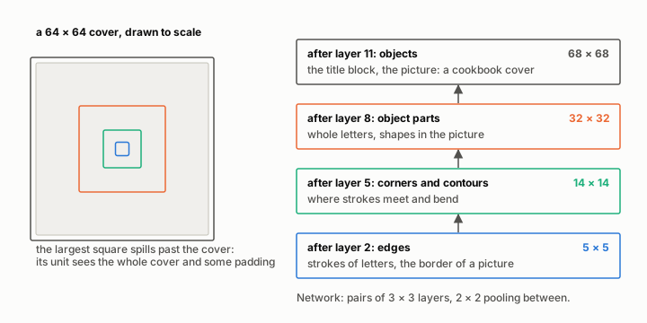 Figure 21.3. The visual hierarchy with its field sizes. After layers 2, 5, 8 and 11 of a small network, units see 5 × 5, 14 × 14, 32 × 32 and 68 × 68 pixels of a 64 × 64 cover.
Real networks follow the same pattern at a larger scale. GoogLeNet takes 224 × 224 images, shrinks its grid to 7 × 7 by its last block while its channels grow from 64 after the first layer to 1,024, and then averages each 7 × 7 channel into one number, so every channel describes the whole image (Szegedy and colleagues, Table 1). At the 7 × 7 stage neighbouring units are 32 pixels apart, since 224 ÷ 7 = 32. The article in my notes read this as each unit representing a 32 × 32 patch, but 32 is the jump, not the field. Araujo and colleagues compute receptive fields from 195 pixels (for a version of AlexNet) to 3,039 (for Inception-ResNet v2), all with that same jump of 32.
Small kernels, stacked
Stacking small kernels is also cheaper than using one large kernel. Simonyan and Zisserman’s VGG paper points out that two 3 × 3 layers see a 5 × 5 region with 18 weights per pair of channels instead of 25, and three see 7 × 7 with 27 instead of 49; one 7 × 7 layer needs 81% more. Each extra layer also brings its own ReLU, so the stack can respond in more complicated ways (Figure 21.4).
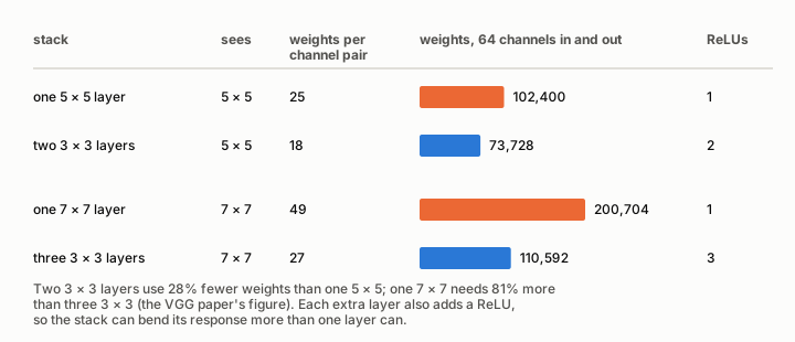 Figure 21.4. Small kernels stacked. Two 3 × 3 layers see 5 × 5 with 73,728 weights for 64 channels, against 102,400 for one 5 × 5; three 3 × 3 layers use 110,592 against 200,704 for one 7 × 7.
Watch, read, try
- Receptive field — Alonso and Chen’s Scholarpedia article on receptive fields in the brain.
- Receptive fields — a physiology lecture on receptive fields.
- Understanding the receptive field of deep convolutional networks — Nikolas Adaloglou’s AI Summer article, saved beside the passage above.
- Unveiling the Impact of Kernel Size on Convolutional Neural Network Architectures — the Kaggle post my notes pasted, with the one-step formula.
Check yourself. 1. What is the receptive field of two stacked 3 × 3 layers with stride 1? 2. A 3-wide layer follows two layers that each have kernel 2 and stride 2. How many input pixels does it see? 3. Why does the centre of a receptive field influence a unit more than its edge?
Answers. 1. 5 × 5. 2. Twelve: the first layer gives r = 2 and j = 2, the second r = 2 + 1 × 2 = 4 and j = 4, the third r = 4 + 2 × 4 = 12. 3. Many more paths through the layers start at the centre, so its signal, and its gradient, travel by more routes.
22. 1×1 convolutions, dilation and separable convolutions
In one breath. Three variations on the convolution change what it costs and what it sees: a 1 × 1 kernel mixes channels without looking at neighbours, a dilated kernel spreads its taps to see further, and a separable convolution splits one expensive step into two cheap ones. Most efficient modern image networks are built from them.
1 × 1: mixing channels
A 1 × 1 convolution looks at a single pixel, but at all of its channels at once. Each 1 × 1 filter takes a weighted sum of the channel values at a pixel, and it does so at every pixel with the same weights, so it acts like a small dense layer applied position by position. Lin, Chen and Yan’s “Network in Network” paper of 2013 made this idea popular. In Figure 22.1, a pixel with red, green and blue values 2, 1 and 0 meets two 1 × 1 filters with weights (1, 1, 0) and (0, −1, 2), and becomes two numbers, 3 and −1. Three channels in, two out, and the four-by-four layout does not change.
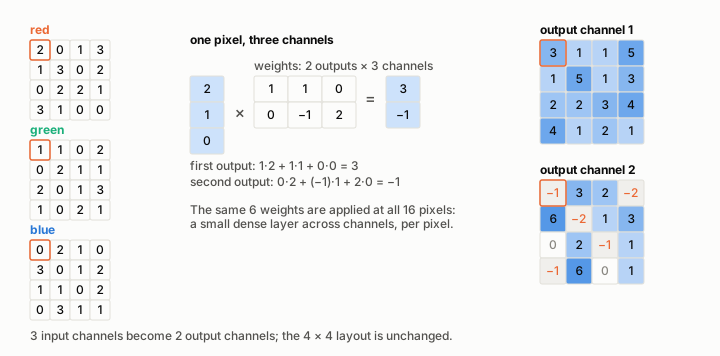 Figure 22.1. A 1 × 1 convolution. The pixel (2, 1, 0) becomes (3, −1); the same six weights at all 16 pixels turn three channels into two.
The main use is to shrink the number of channels before an expensive convolution. GoogLeNet, a network 22 layers deep that won the 2014 ImageNet challenge with a top-5 error of 6.67%, puts 1 × 1 reductions in front of its 3 × 3 and 5 × 5 convolutions, each followed by its own ReLU (Szegedy and colleagues, 2015). Figure 22.2 shows the saving on a 28 × 28 map with 256 channels: a 3 × 3 convolution straight to 128 channels costs 231,211,008 multiplications, while a 1 × 1 step down to 64 channels followed by the 3 × 3 convolution costs 12,845,056 + 57,802,752 = 70,647,808, or 30.6% as much. ResNet’s deeper versions use the same trick in their “bottleneck” blocks, with a 1 × 1 layer before and after each 3 × 3: the first reduces 256 channels to 64, and the last restores 256. A 1 × 1 layer can widen as easily as it narrows, and because a nonlinearity follows it, a stack of them acts like the small network at every pixel that gave Lin, Chen and Yan’s paper its name.
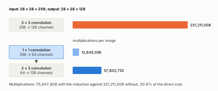 Figure 22.2. A 1 × 1 reduction before a 3 × 3 convolution on a 28 × 28 × 256 input: 70,647,808 multiplications against 231,211,008, 30.6% of the direct cost.
Dilation: seeing further with the same weights
A dilated kernel spreads its taps apart, leaving d − 1 empty pixels between neighbouring taps for a dilation rate d. A 3 × 3 kernel then spans k + (k − 1)(d − 1) pixels: 5 × 5 at dilation 2 and 9 × 9 at dilation 4, still with nine weights (Dumoulin and Visin). Stacking dilations of 1, 2 and 4 gives fields of 3, 7 and 15 without ever shrinking the image (Figure 22.3). Yu and Koltun (2016) used such stacks to let a network see wide context while keeping every output pixel, which matters when the task is to label every pixel of an image. Dilation works along time as well: Dumoulin and Visin point to WaveNet, a model of raw audio that stacks dilated convolutions so that each new sound sample can depend on a long stretch of the samples before it. This growth happens inside single layers, unlike the growth after a stride in chapter 21.
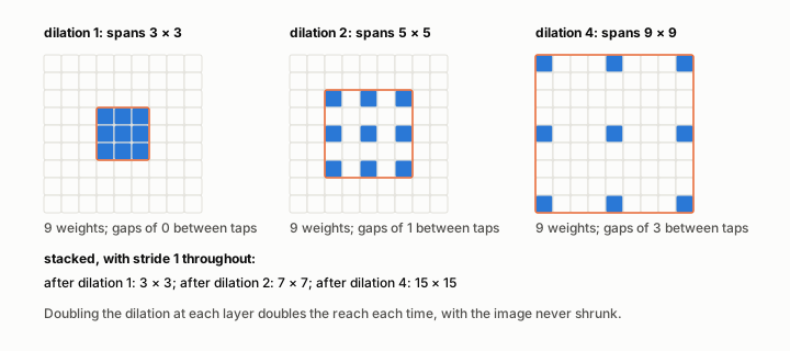 Figure 22.3. Dilation spreads nine taps over 3 × 3, 5 × 5 and 9 × 9 pixels; stacked with dilations 1, 2 and 4 the layers see 3 × 3, 7 × 7 and 15 × 15.
Separable convolutions
Some kernels can be written as a column times a row. The Sobel kernel of chapter 19 is the column (1, 2, 1) times the row (1, 0, −1), so convolving with the column and then with the row gives the same result as the full kernel, at 6 multiplications per pixel instead of 9 (Figure 22.4, right). This is a spatially separable kernel.
The version that matters more in practice is the depthwise separable convolution. It splits a standard convolution into a depthwise step, one 3 × 3 kernel per input channel with no mixing between channels, followed by a pointwise step, a 1 × 1 convolution that does all the mixing (Chollet, 2017; Howard and colleagues, 2017). For a 56 × 56 map with 64 channels in and 128 out, the standard convolution costs 231,211,008 multiplications, and the two steps together cost 1,806,336 + 25,690,112 = 27,496,448, which is 0.119 of the standard cost. Howard and colleagues give the ratio as 1/N + 1/k² for N output channels and a k × k kernel, here 1/128 + 1/9. The weights shrink in the same way, from 73,728 to 8,768. MobileNets use 3 × 3 depthwise separable convolutions throughout and report 8 to 9 times less computation for a small loss of accuracy. Chollet arrived at the same split from the other direction: he describes a depthwise separable convolution as an Inception block taken to its extreme, with the largest possible number of branches, and his Xception network, built that way, matches Inception V3’s parameter count and does slightly better on ImageNet.
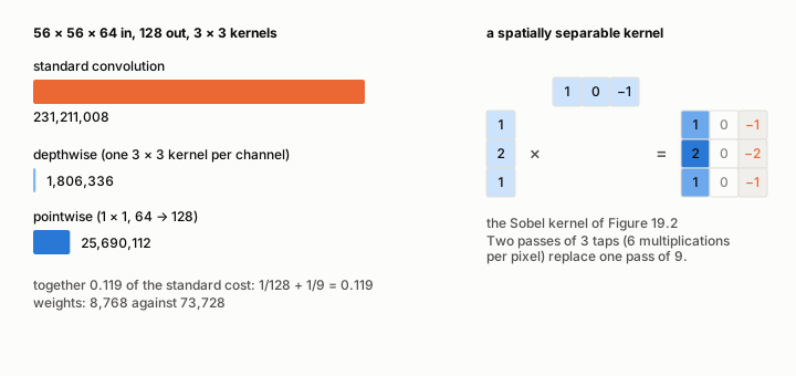 Figure 22.4. Separable convolutions. Depthwise plus pointwise steps cost 27,496,448 multiplications against 231,211,008, a ratio of 0.119 = 1/128 + 1/9; the Sobel kernel is a column times a row.
Watch, read, try
- A Gentle Introduction to 1x1 Convolutions to Manage Model Complexity — Jason Brownlee on using 1 × 1 filters to cut channels.
- C4W2L07 Inception Network — Andrew Ng’s lecture on the Inception network.
- Going Deeper with Convolutions — the GoogLeNet paper.
- What’s the use of dilated convolutions? — a Stack Overflow thread pointing to Yu and Koltun’s context module.
- A Basic Introduction to Separable Convolutions — an introductory article on separable convolutions.
Check yourself. 1. How many weights does a 1 × 1 convolution from 256 channels to 64 channels need, ignoring biases? 2. How many pixels does a 3 × 3 kernel with dilation 3 span? 3. For a 3 × 3 depthwise separable convolution with 128 output channels, about what fraction of the standard cost remains?
Answers. 1. 256 × 64 = 16,384. 2. 3 + 2 × 2 = 7 pixels across, a 7 × 7 span. 3. About 1/128 + 1/9 ≈ 0.119, roughly an eighth.
23. Squeeze-and-Excitation, skip connections, and what CNNs get wrong
In one breath. Two small additions made convolutional networks much better: squeeze-and-excitation lets a network turn each channel up or down according to the whole image, and skip connections let very deep networks train at all. Yet a network that names pictures superbly can be fooled by changes a person cannot see, a reminder that recognising is not the same as understanding.
Squeeze-and-excitation
A convolution sees only a small window, so no single unit knows what the whole image contains. The squeeze-and-excitation (SE) block of Hu, Shen and Sun (2018) adds that knowledge cheaply, in three steps. Squeeze: average each channel over all its positions, which gives one number per channel. Excite: pass those numbers through two small layers, one that shrinks them by a reduction ratio and applies ReLU, and one that expands them back, then a sigmoid, which gives one gate between 0 and 1 per channel. Scale: multiply every position of each channel by its gate.
Figure 23.1 runs the steps on three small channels. Their averages are 4, 2 and 1; the first small layer turns them into a single hidden number, 1.75; the second layer and the sigmoid give gates of 0.891, 0.259 and 0.587; and each channel is scaled by its gate, so channel 1 keeps most of its strength and channel 2 is turned well down.
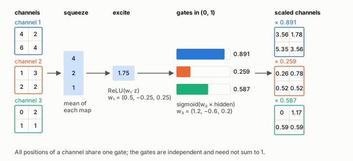 Figure 23.1. A squeeze-and-excitation block. Averages 4, 2 and 1 give a hidden value of 1.75 and gates 0.891, 0.259 and 0.587, which rescale the three channels.
The cost is small: with a reduction ratio of 16, SE-ResNet-50 needs 3.87 billion floating-point operations against 3.86 billion for ResNet-50. The gain was large: SE networks won the 2017 ImageNet classification challenge with a top-5 error of 2.251%, about a quarter lower in relative terms than the previous year’s winner. The authors chose a sigmoid so that several channels can be emphasised at once instead of a single one winning; the gates do not have to add up to one.
From my notes. Question: is squeeze-and-excitation an attention mechanism? Answer: it uses an attention-like gate; it is not self-attention.
That answer holds up. Hu and colleagues describe the excitation as a simple self-gating mechanism and the whole block as a lightweight gate, and it does resemble attention in that it decides what to emphasise. But it never compares positions with each other. Self-attention scores every position against every other position and mixes their contents; an SE block summarises each channel into one number and rescales whole channels.
Skip connections
In 2015 Kaiming He and colleagues observed that stacking more and more layers made networks worse, and not through overfitting: a plain network of 56 layers had a higher error on its own training images than one of 20 layers (their Figure 1). Their fix was the residual block of Figure 23.2. A skip connection carries the block’s input x around its layers and adds it to their output, so the block computes F(x) + x, and its layers learn F(x), the change to make, rather than the whole mapping. If the best thing a block can do is leave its input alone, a plain block has to learn an exact copy through two convolutions and a ReLU, while a residual block only has to push its weights to zero.
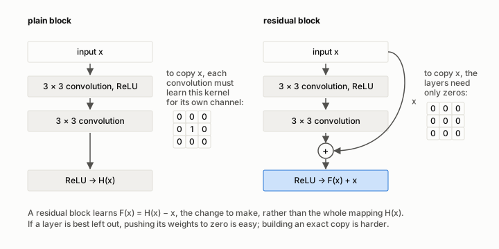 Figure 23.2. A plain block and a residual block. To pass its input through unchanged, the plain block must learn the identity kernel in each convolution; the residual block needs only zeros, since F(x) = 0 gives F(x) + x = x.
With these blocks He and colleagues trained networks 152 layers deep, eight times deeper than VGG, and an ensemble of them, several networks whose predictions are combined, reached a top-5 error of 3.57% on the ImageNet test set, winning the 2015 challenge.
From my notes. ResNet: for the deeper layers it is easier to learn the zero function than the identity function.
This is the heart of the ResNet paper, in one line. The authors put it as a hypothesis: if an identity mapping were the best choice, it would be easier to push the residual to zero than to fit the identity with a stack of nonlinear layers.
What CNNs get wrong
Ian Goodfellow, Jonathon Shlens and Christian Szegedy (2015) took a photo that GoogLeNet labelled “panda” with 57.7% confidence, changed every pixel by 0.007 in the direction that increases the network’s error, and got “gibbon” with 99.3% confidence, although the two images look identical to a person. Such adversarial examples do not need a mysterious cause. For a linear score, a nudge of size ε to each of n inputs, each in the direction of its weight, changes the score by ε × m × n, where m is the average size of a weight. The change grows with the number of pixels. Figure 23.3 works it with ε = 0.007 and an assumed m of 0.01: about 0.003 for our 36-pixel cover, but about 10.5 for a 224 × 224 colour photo, easily enough to swap one label for another.
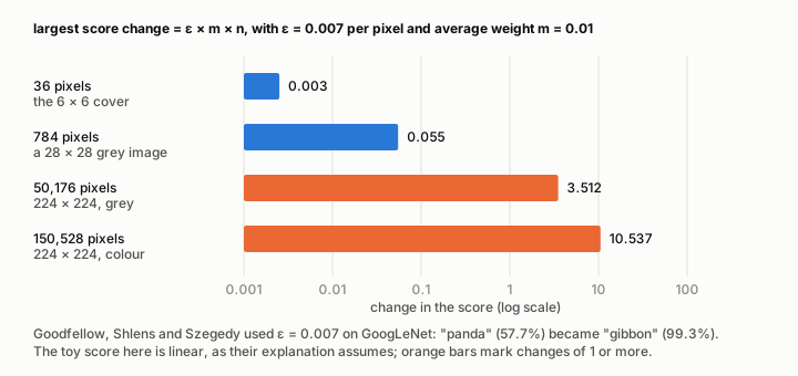 Figure 23.3. Many tiny changes add up. With ε = 0.007 per pixel and an average weight of 0.01, a linear score can move 0.003 for 36 pixels, 3.512 for 50,176 and 10.537 for 150,528.
The article in my notes adds a broader warning: a network can recognise the objects in a photo without grasping the scene, and it cites a case in which Facebook removed a post showing the Venus of Willendorf, a small stone figure about 29,500 years old, as nudity. Vienna’s Natural History Museum protested, and Facebook apologised on 1 March 2018, according to an AFP report; that report does not say whether a person or a program made the decision, so the story is a caution about automated judgement in general rather than evidence about convolutional networks in particular.
Watch, read, try
- ResNet (actually) explained in under 10 minutes — a short explanation of ResNet.
- Deep Residual Learning for Image Recognition (Paper Explained) — Yannic Kilcher reads the ResNet paper in his series on classic papers; from 7:26, the point my notes saved.
- Attacking Machine Learning with Adversarial Examples — OpenAI’s 2017 post by Goodfellow and colleagues; the old address now redirects to OpenAI’s news page.
- How to train an ensemble of convolutional neural networks for image classification — a tutorial on combining several networks, as the ImageNet winners did.
Check yourself. 1. What does the squeeze step compute? 2. Why does a residual block find it easy to leave its input unchanged? 3. Why do adversarial nudges become more dangerous as images get larger?
Answers. 1. The average of each channel over all its positions, one number per channel. 2. With all its layer weights at zero, F(x) = 0 and the block outputs F(x) + x = x. 3. The largest change in a linear score is ε × m × n, which grows with the number of pixels n even when each pixel’s change stays tiny.
24. Convolution beyond images
In one breath. Convolution is not only an image operation: it is also how two probability distributions combine when their quantities are added, as when two customers’ book counts add up to a total. Seeing it this way explains the flip in the textbook definition, and why deep-learning libraries can leave it out.
Two customers come in, and each buys between one and six books with the probabilities of chapter 12: 0.35 for one book, 0.275 for two, down to 0.05 for six. If they choose independently, how likely is it that they buy five books between them? The total is 5 in four ways: 1 and 4, 2 and 3, 3 and 2, or 4 and 1. Each way has probability equal to the product of its two parts, and the four products add up:
0.35 × 0.1 + 0.275 × 0.175 + 0.175 × 0.275 + 0.1 × 0.35 = 0.16625.
Doing this for every total from 2 to 12 gives the whole distribution of the total, drawn in Figure 24.1. Its eleven bars add up to 1, and the most likely total is 4. The shape is worth a second look. On average one customer buys 2.375 books, and two customers buy 4.75 between them, exactly twice as many. The most likely single basket, though, is one book, while the most likely total is not two but four, because so many different pairs lead to the middle totals and only one pair, one book each, leads to two.
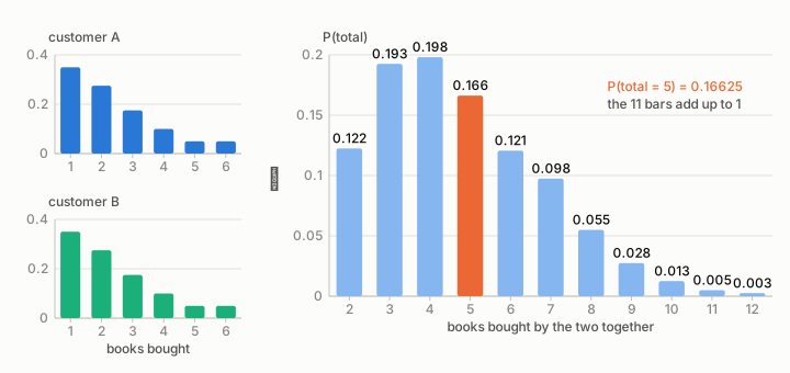 Figure 24.1. The distribution of the total is the convolution of the two customers’ distributions. P(total = 5) = 0.16625, and the eleven bars add up to 1.
In general, for two independent quantities that take whole-number values, the chance of a total t is
\[P(A + B = t) = \sum_{x} P(A = x)\, P(B = t - x)\]and this operation on the two lists of probabilities is called convolution. For a pair of fair dice the same sum gives the familiar 6 chances in 36, or 1/6, of throwing a 7.
Flip and slide
Look at the pairs again: as A’s count x goes up, B’s count t − x goes down. To line the pairs up, write A’s probabilities left to right and B’s right to left, the flip, and shift B’s reversed list along A’s until the pairs you want sit on top of each other, the slide. Multiply the pairs that overlap and add (Figure 24.2). Each step to a larger total slides B’s list further to the right. 3Blue1Brown’s video on sums of random quantities, which my notes screenshotted, draws the same flip-and-slide picture.
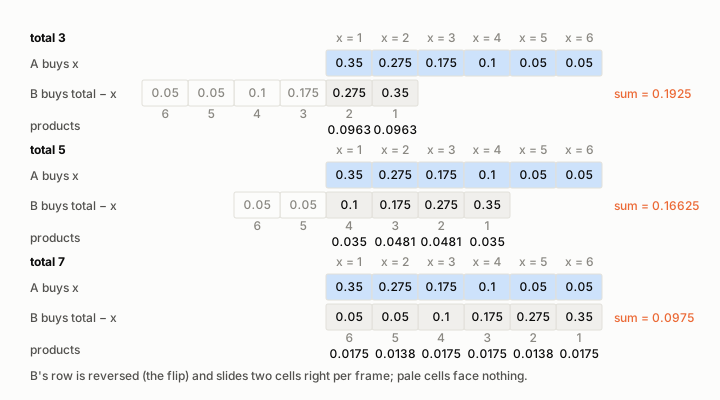 Figure 24.2. Flip and slide. Reversing B’s probabilities and sliding them under A’s gives 0.1925 for a total of 3, 0.16625 for 5 and 0.0975 for 7.
The same arithmetic turns up in algebra. The coefficients of the product of two polynomials are the convolution of their coefficient lists, a rule known as the Cauchy product. Write the basket probabilities as 0.35z + 0.275z² + 0.175z³ + 0.1z⁴ + 0.05z⁵ + 0.05z⁶, multiply the polynomial by itself, and the coefficient of z⁵ is 0.16625, the chance of a total of five.
For quantities that vary continuously, such as the time two customers spend browsing, the sum becomes an integral of one density times the other, reversed and shifted. 3Blue1Brown’s rule of thumb, saved as a screenshot in my notes, is that sums in the whole-number case become integrals in the continuous case.
Back to images, and to time
Convolutions also run along time. Smoothing the shop’s daily sales with a three-day average is a convolution with the kernel (1/3, 1/3, 1/3): sales of 4, 6, 5, 9 and 7 books become 5, 6.67 and 7, each the mean of three neighbouring days. Networks for sound and other signals use such one-dimensional convolutions with learned kernels, and the dilated stacks of chapter 22 let them look far back in time. A simple blur of a photo is the two-dimensional version of the same average: a kernel of equal weights that add up to one, slid over the image, so that every pixel becomes the mean of its neighbourhood.
The image convolution of chapter 17 is the same operation in two dimensions: a small grid of weights, flipped and slid over a larger grid, multiplying and adding. Deep-learning libraries skip the flip and compute what mathematicians call cross-correlation, as Goodfellow, Bengio and Courville note. Nothing is lost, because a kernel that is learned can learn its weights in the flipped order equally well, and Dumoulin and Visin make the same remark. In probability the flip matters, because the lists are given and their order carries meaning: B’s list must run backwards for the pairs to add up to the total.
Watch, read, try
- But what is a convolution? — 3Blue1Brown’s introduction to convolution.
- Convolutions, Why X+Y in probability is a beautiful mess — 3Blue1Brown on sums of random variables, from 2:13, the point my notes saved.
Check yourself. 1. With the basket probabilities, what is the chance that the two customers buy two books between them? 2. Why is B’s list reversed in Figure 24.2? 3. What replaces the sum when the two quantities are continuous?
Answers. 1. Only one way, one book each: 0.35 × 0.35 = 0.1225. 2. For a fixed total, a larger count for A means a smaller count for B, so B’s values must run in the opposite direction for the pairs to line up. 3. An integral of one density times the other, reversed and shifted.
Part V: Words as numbers: embeddings
25. From one-hot to embeddings
In one breath. A program can only work with numbers, so every word it reads must first become a list of numbers. An embedding is a short list chosen so that words with related meanings get related lists, and that one idea is what lets a machine see that a detective story and a mystery belong on the same shelf.
Your shop sells stories, cookbooks and repair manuals, and in the window you have pinned five blurbs, the short descriptions from the back covers. This part of the book uses them as its text:
| Blurb | Text |
|---|---|
| B1 | a quiet mystery in a small town |
| B2 | a small town detective and a quiet mystery |
| B3 | recipes from a village kitchen |
| B4 | the detective returns to the village |
| B5 | how to repair a bicycle |
You can tell at a glance that B1, B2 and B4 describe the same kind of book. A program cannot. To a program a word is a string of letters with no meaning attached, and before it can learn anything each word has to become numbers in a way that keeps some of that meaning.
One column per word
The plainest method is one-hot encoding. List every word you might meet (this list is the vocabulary), give each word its own column, and write a word as a row of zeros with a single 1 in its own column. The left half of Figure 25.1 does this for the eleven content words of the blurbs.
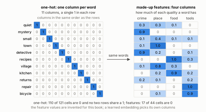 Figure 25.1. The eleven content words of the blurbs, once as one-hot rows (110 of 121 cells are 0, and no two rows share a 1) and once as four made-up features (17 of 44 cells are 0). The feature values were set by hand for this book.
One-hot codes are honest but blind. Two different words never have their 1 in the same column, so multiplying their rows entry by entry and adding up, the dot product of chapter 4, always gives 0, and the straight-line distance between them is always the square root of 2. “Mystery” is exactly as far from “detective” as it is from “bicycle”. The rows are also long. The scikit-learn documentation gives a feel for real sizes: ten thousand short texts such as e-mails can use about 100,000 different words between them, so each word would be a row of 100,000 numbers holding a single 1. A row like that is sparse, meaning almost all of its entries are zero.
Columns that mean something
Now describe the same words by their qualities instead. The right half of Figure 25.1 gives each word four numbers between 0 and 1, one for each of four made-up features: how much the word has to do with crime, with a place, with food and with tools. I chose these values by hand so that you can read them; nothing learned them. “Mystery” becomes (0.9, 0, 0, 0) and “detective” (0.9, 0.2, 0, 0.1), close to each other and far from “recipes” at (0, 0, 1.0, 0.3).
A list like this is dense: short, with most entries non-zero. An embedding is a dense list of numbers that stands for an object, arranged so that similar objects get similar lists. In a 2019 answer on Data Science Stack Exchange, the user sdaylor calls it “a low-dimensional, learned continuous vector representation of discrete variables”. Each word of that definition carries weight. Low-dimensional means few numbers. Learned means a training process sets them; setting them by hand, as here, is the one liberty this chapter takes. Continuous means any value, not only 0 or 1.
To measure how alike two such lists are, the usual tool is cosine similarity, the cosine of the angle between the two vectors: 1 when they point the same way, 0 when they meet at a right angle. Chapter 27 looks at it closely. With the four features, mystery and detective score 0.97, town and village 0.94, and mystery and recipes exactly 0, because they share no feature at all. With one-hot codes every one of those pairs scores 0.
Four numbers per word cannot be drawn on a page, so Figure 25.2 uses the two directions along which the eleven words spread out most, found by principal component analysis, the subject of chapter 29. Together those two directions keep 73% of the spread. The crime words, the place words, the food words and the tool words gather in four separate corners, with vaguer words such as “quiet” and “returns” nearer the middle.
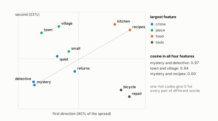 Figure 25.2. The feature vectors of Figure 25.1 flattened onto their two main directions, which keep 40% and 33% of the spread. Cosine similarity in all four features: mystery and detective 0.97, town and village 0.94, mystery and recipes 0.00.
An embedding layer is a lookup table
A network uses such a table in the simplest possible way. Multiply a one-hot row by the table, and the single 1 keeps one row of the table while every 0 wipes out its row. Figure 25.3 shows this for “detective”: the product is detective’s own row, (0.9, 0.2, 0, 0.1). An embedding layer, the first layer of every language model in this book, is therefore a table with one row per vocabulary word, and “embedding a word” means reading its row. A program can read the row directly and skip the multiplication, and the answer is the same.
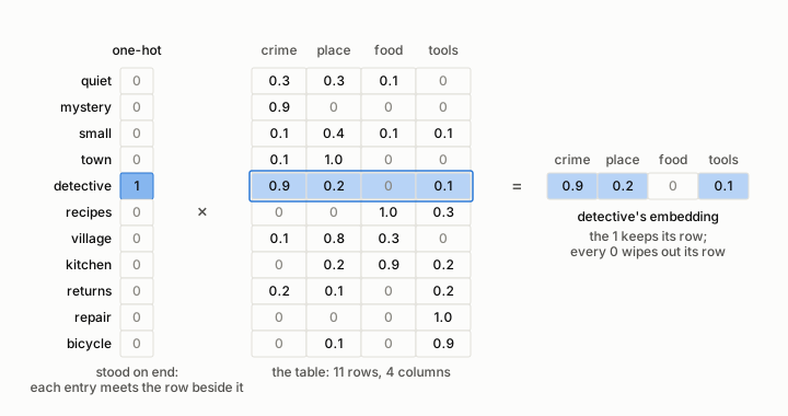 Figure 25.3. Multiplying the one-hot code of detective by the feature table returns detective’s own row, (0.9, 0.2, 0, 0.1). The one-hot row is drawn standing on end so that each entry sits beside the row it multiplies.
In a real model nobody fills the table in. It starts as small random numbers and is adjusted during training, a little at a time, so that the whole network gets better at its task, such as guessing a missing word. The columns that emerge usually have no names like “crime” or “food”; they are whatever directions happened to help. Chapters 27 and 28 show two ways of learning such a table from plain text.
Anything can be embedded
The same idea works for any object whose likeness you care about: a blurb, a whole review, a photograph of a cover. An embedding model takes the object, whatever its size, and returns a vector of one fixed length (Figure 25.4). The sentence-transformers model all-MiniLM-L6-v2, for instance, turns an English text into 384 numbers, and the same library lists models such as CLIP that place photographs and captions in one shared space. Comparing two objects then becomes comparing two vectors, which is cheap. The library’s documentation names semantic search, finding texts by meaning rather than by shared words, and paraphrase mining, finding texts that say the same thing, among the uses.
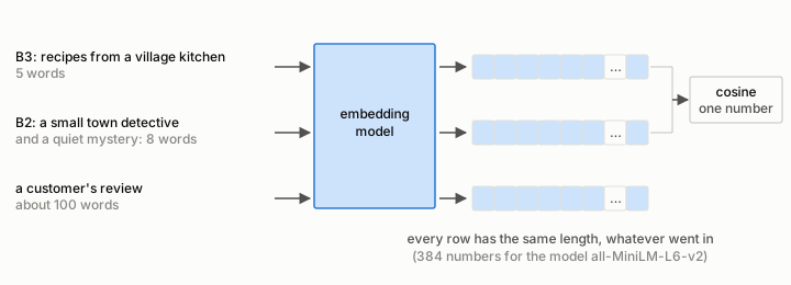 Figure 25.4. An embedding model returns a vector of the same length for every input, 384 numbers in the case of all-MiniLM-L6-v2; comparing two texts then means comparing two vectors.
Watch, read, try
- Google Machine Learning Crash Course: Embeddings — a 45-minute module on why one-hot vectors fall short and how embeddings fix them.
- An Introduction to Graph Neural Networks, Microsoft Research — the saved moment (49:23) contrasts a one-hot “local” code with a dense, distributed one written as a matrix times a one-hot vector.
- AWS: What are embeddings in machine learning? — a plain overview with a one-hot table of fruit prices and a made-up example of television programmes.
- What does embedding mean in machine learning? (Data Science Stack Exchange) — sdaylor’s short accepted answer, quoted in this chapter.
- A guide on word embeddings in NLP (Turing) — the guide my notes pasted in full: TF-IDF, bag of words, Word2Vec, GloVe and BERT in one long page, with code.
Check yourself. 1. What is the cosine similarity between the one-hot codes of “town” and “village”, and why? 2. Judging by the four features of Figure 25.1, is “village” closer to “town” or to “kitchen”? 3. In Figure 25.3, what would you get by multiplying the one-hot code of “repair” by the table?
Answers. 1. It is 0: the two rows never have a 1 in the same column, so their dot product, and with it the cosine, is 0. 2. To “town”: the two share a large place value and little else, while most of kitchen’s weight is food. 3. Repair’s own row, (0, 0, 0, 1.0).
26. Counting words: bag of words and TF-IDF
In one breath. The oldest way to turn a text into numbers is to count how often each word occurs in it, and then to weigh each count by how rare the word is across all your texts. The resulting vectors are long, mostly empty and blind to word order, but they are quick, easy to explain and still used in search.
A bag of words
Before counting, a text is split into tokens, the pieces a program treats as units. Here a token is a word, found by splitting on spaces after turning everything to lowercase. The bag of words of a text records how many times each vocabulary word occurs in it. The name fits: tip the words into a bag, shake it, and keep only how many of each you have.
Figure 26.1 shows the bags of the five blurbs. Their vocabulary has 18 words, so each blurb becomes a column of 18 counts. B1 and B2 each contain “a” twice and B4 contains “the” twice; every other count is 0 or 1. Of the 90 cells, 62 are zero, which is 69%. Real collections are far emptier. The scikit-learn documentation describes 10,000 short texts that use about 100,000 different words between them while each text uses somewhere between 100 and 1,000, so that more than 99% of such a table is typically zero.
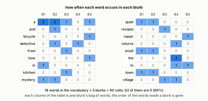 Figure 26.1. The bag of words of each blurb, one column per blurb. Only “a” (in B1 and B2) and “the” (in B4) occur twice; 62 of the 90 cells are 0.
Counts already say something. The cosine similarity between the count columns of B1 and B2 is 0.84, because the two blurbs share quiet, mystery, small, town and two copies of “a”. The left half of Figure 26.3 shows the trouble, though. B1 scores 0.30 with the recipe blurb B3 and exactly the same 0.30 with the bicycle blurb B5, and in both cases the whole resemblance comes from the little word “a”.
Rare words matter more
The term frequency (tf) of a word in a text is how often it occurs there: its count. Its document frequency (df) is the number of texts in the collection that contain it at least once. A word found in nearly every text, like “a”, tells you little about any one of them; a word found in a single text tells you a lot. The inverse document frequency (idf) turns that into a number. The information-retrieval textbook of Manning, Raghavan and Schütze defines it as the logarithm of the number of texts divided by the document frequency, and I use the natural logarithm, ln:
\[\text{idf} = \ln \frac{\text{number of texts}}{\text{number of texts that contain the word}}\]The tf-idf weight of a word in a text is its count multiplied by its idf. The same textbook points out that the base of the logarithm does not change which texts rank above which.
Figure 26.2 works this out for B1. The word “a” occurs twice in B1, but four of the five blurbs contain it, so its idf is ln(5 ÷ 4) = 0.223 and its weight only 0.446. “Quiet”, “mystery”, “small” and “town” each appear in two blurbs and weigh 0.916. The heaviest is “in”: it occurs in B1 alone, so it gets the full ln 5 = 1.609. That last result is a warning, not a triumph. In five short blurbs the little word “in” happens to be rare, and tf-idf cannot tell rarity from importance. This is why most systems first remove stop words, common words such as “and”, “the” and “in”; scikit-learn’s documentation describes them as words “presumed to be uninformative in representing the content of a text”.
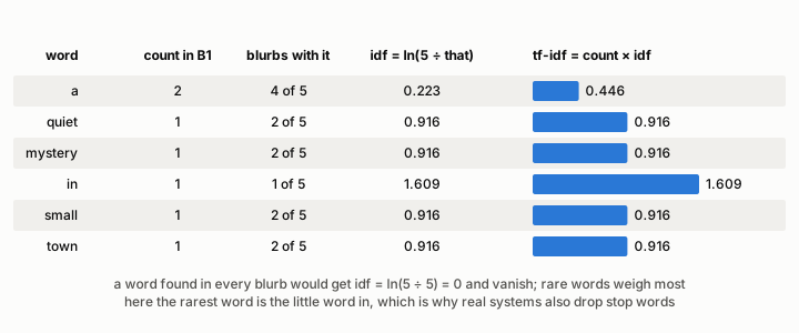 Figure 26.2. tf-idf for blurb B1: “a” occurs twice but is in four of the five blurbs, so it weighs only 0.446; “in” occurs once but in B1 alone, so it weighs 1.609.
With tf-idf weights in place of raw counts, the false likeness through “a” almost disappears. In the right half of Figure 26.3, B1 and B5 fall from 0.30 to 0.01, and B1 and B3 do the same. B1 and B2 drop as well, from 0.84 to 0.54, because the words they share are not rare, but they stay by far the closest pair.
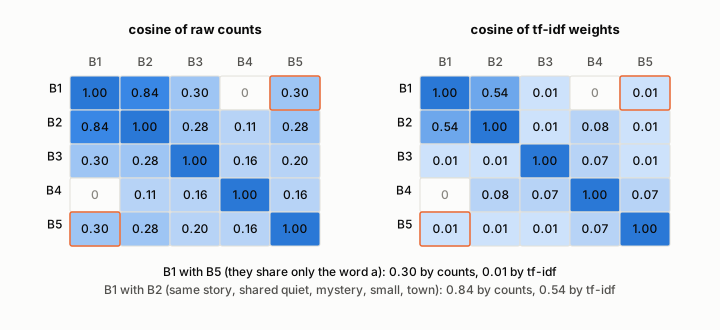 Figure 26.3. Cosine similarity between the blurbs. B1 and B5 share only “a”: 0.30 by counts, 0.01 by tf-idf. B1 and B2 share four content words: 0.84 by counts, 0.54 by tf-idf. B1 and B4 share nothing: 0 either way.
Libraries use small variations on these formulas. The TfidfTransformer of scikit-learn, for instance, by default adds 1 to both counts inside the logarithm and 1 to the result, and then scales each text’s vector to length 1, so its numbers differ from Figure 26.2 while the idea is unchanged. The Turing guide in the list below uses another common variant, dividing each count by the length of its text.
What counting cannot see
Counts ignore order. Figure 26.4 turns B4 back to front: “the village returns to the detective” tells a different story, yet its bag is identical, count for count. Counts also know nothing of meaning. B1 and B4 are both small-town crime stories, but they share no word, so every count-based similarity between them is 0. And the vectors grow with the vocabulary, one entry for every word ever seen. Embeddings, built in the next three chapters, deal with the last two problems; order has to wait for position codes in chapter 31.
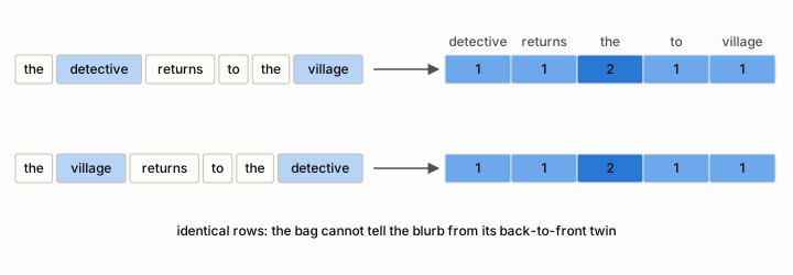 Figure 26.4. Reversing blurb B4 changes the story but not a single count: a bag of words cannot see order.
Watch, read, try
- spaCy vs NLTK (Konfuzio) — two Python toolkits that do the tokenising and stop-word removal described here.
Check yourself. 1. What is the idf of “detective” in the five blurbs? 2. Why does “in” get the largest tf-idf weight in B1? 3. Write a different phrase with exactly the same bag of words as B1.
Answers. 1. It is ln(5 ÷ 2) = 0.916, the same as for any word found in two of the five blurbs. 2. Because it occurs in B1 alone; idf rewards rarity, and in five short blurbs a little word can be rare. 3. For example, “a small mystery in a quiet town”.
27. Word2Vec: CBOW and skip-gram
In one breath. Word2Vec learns an embedding table by playing a guessing game: predict a word from its neighbours, or the neighbours from the word. Words that keep the same company end up with similar vectors, because similar vectors make the same guesses easy.
In 2013 Tomas Mikolov and his colleagues at Google published two papers describing a fast way to learn word vectors from plain text. The method bets on one plain observation: words that turn up in the same surroundings tend to mean related things. It never looks up a definition. It only watches which words keep company.
The window
A context window is a few words on each side of a centre word. Figure 27.1 slides a window of two words on each side along B2. With “detective” in the centre, the four neighbours are “small”, “town”, “and” and “a”. Near the end, with “quiet” in the centre, the window is cut short and holds only “and”, “a” and “mystery”. Every (centre, neighbour) pair is one training example, and sliding the window over all five blurbs gives 94 of them.
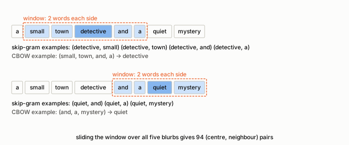 Figure 27.1. A window of two words on each side turns B2 into training pairs; near the end of the blurb the window is cut short. All five blurbs together give 94 pairs.
Two guessing games
CBOW, short for continuous bag of words, looks up the rows of the neighbours in the embedding table, averages them into one vector, scores every word of the vocabulary against that average and turns the scores into probabilities. Training nudges the numbers so that the true centre word, “detective”, becomes more probable. Skip-gram plays the game the other way round: it looks up the centre word’s row alone and asks it to predict each neighbour in turn. Figure 27.2 draws both. In the first paper, CBOW trained faster (about a day against about three on the same subset of data), while skip-gram did better on the questions about meaning.
The step that turns scores into probabilities is softmax. Raise the number e to the power of each score, then divide each result by their total, so that every value is positive and they add up to 1:
\[\text{softmax}(s)_i = \frac{e^{s_i}}{\sum_j e^{s_j}}\]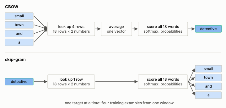 Figure 27.2. The two Word2Vec games on one window of B2. Both look words up in the same table of 18 rows; both score all 18 words and apply softmax.
Scoring every word is costly when the vocabulary holds a million words, the size used in the first paper, so the papers took shortcuts. The first arranged the vocabulary in a tree, a so-called hierarchical softmax; the second offered a simpler alternative, negative sampling: for each true pair, draw a few random “noise” words and train the model only to tell the true neighbour from them. The authors found 5 to 20 noise words useful for small data sets and as few as 2 to 5 for large ones.
Where the embedding lives
The table the model looks words up in is the embedding. To make that concrete I trained a tiny skip-gram on the five blurbs, with only two numbers per word so that the whole table fits in Figure 27.3. It is the full-softmax version described above, with a window of two, 3,000 passes over the 94 pairs and small random starting values. The one-hot code of “mystery” picks out its row, (−0.42, −3.25). On its own that pair of numbers means nothing; only its relation to the other rows does.
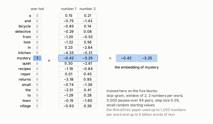 Figure 27.3. The embedding table of a tiny skip-gram trained on the five blurbs (two numbers per word, window 2, 3,000 passes over 94 pairs). The one-hot code of mystery picks out its row, (−0.42, −3.25).
Reading angles: cosine similarity
For two vectors a and b, the cosine similarity is their dot product divided by the product of their lengths:
\[\cos\theta = \frac{a \cdot b}{\lVert a \rVert \, \lVert b \rVert}\]It is 1 when the vectors point the same way, 0 when they meet at a right angle and −1 when they point in opposite directions (Figure 27.4, left). Because it divides by the lengths, only direction counts.
On the right of Figure 27.4 are six rows of the trained table. Mystery and town point almost exactly the same way, with a cosine of 0.999: in the blurbs both always follow “a quiet” or “a small”, so to skip-gram they are the same kind of word. Quiet and small, which both sit between “a” and a noun, score 0.819. Recipes and kitchen, which only ever appear together in B3, score 0.855, while mystery and kitchen, which never share a blurb, score 0.196.
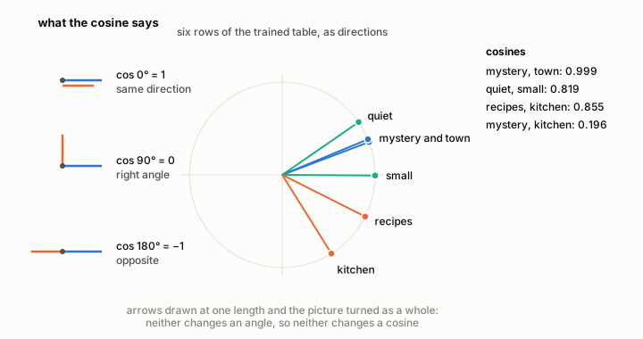 Figure 27.4. Cosine similarity reads angles. In the trained table mystery and town point almost the same way (0.999), quiet and small score 0.819, recipes and kitchen 0.855, and mystery and kitchen 0.196.
The mystery and town result shows the method’s power and its limit together. Skip-gram learns from company alone, and in five blurbs “mystery” and “town” keep identical company, so it cannot tell them apart. I trained the same model from five other random starting points; the rest of the table sometimes changed, but mystery and town ended up pointing the same way (cosine 0.99 or more) every time. With billions of words such accidents average out. The first paper trained vectors of up to 1,000 numbers on up to 6 billion words of Google News, and it recalls the famous result that vector(“King”) − vector(“Man”) + vector(“Woman”) lands closest to vector(“Queen”).
Watch, read, try
- Word Embedding and Word2Vec, Clearly Explained!!! (StatQuest) — Josh Starmer builds the network step by step and shows how to check the result.
- A Complete Overview of Word Embeddings (AssemblyAI) — what word embeddings are, how they are made and how to use them.
- Mikolov et al., Efficient Estimation of Word Representations in Vector Space — the first Word2Vec paper, source of the comparisons in this chapter.
Check yourself. 1. How many (centre, neighbour) pairs does B5, “how to repair a bicycle”, give with a window of two words on each side? 2. Which game, CBOW or skip-gram, looks up a single row for each training example? 3. Two vectors have cosine similarity −1. What does that tell you about them?
Answers. 1. Fourteen: 2 for “how”, 3 for “to”, 4 for “repair”, 3 for “a” and 2 for “bicycle”. 2. Skip-gram, which looks up only the centre word. 3. They point in exactly opposite directions; their lengths can still differ.
28. GloVe: co-occurrence and probability ratios
In one breath. GloVe counts, once and for the whole collection, how often each pair of words appears close together, and then fits word vectors to those counts. Its central insight is that the ratio of two such probabilities says more about meaning than either probability does alone.
Word2Vec reads text window by window. GloVe, from Jeffrey Pennington, Richard Socher and Christopher Manning at Stanford (2014), first tallies every window into one table and then learns from the table. The authors chose the name, Global Vectors, because statistics of the whole corpus feed the model directly. Their paper places GloVe between two older families: methods that factorise one big table of counts for the whole corpus, such as latent semantic analysis, which use the statistics well but do poorly on word analogies, and window-based methods such as skip-gram, which do better on analogies but never look at the corpus-wide counts. GloVe aims to keep the strengths of both.
The co-occurrence table
A co-occurrence matrix has one row and one column per vocabulary word; the entry in row i and column j counts how often word j appears within the window around word i. Figure 28.1 builds it for B1 and B2 with a window of one word on each side. “Quiet” stands next to “a” twice and next to “mystery” twice, so its row holds two 2s. Every neighbouring pair is seen from both ends, which makes the table symmetric; B1 and B2 contain 13 neighbouring pairs between them. The total of a row says how many neighbours that word had altogether.
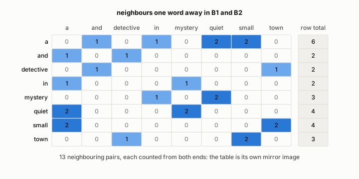 Figure 28.1. Co-occurrence counts for B1 and B2 with a window of one word on each side. The table is symmetric; quiet had 4 neighbours in all, two of them a and two mystery.
Dividing a row by its total gives probabilities. Write P(k given i) for the probability that a neighbour of word i is word k. “Quiet” had four neighbours, two of them “a”, so P(a given quiet) = 2 ÷ 4 = 0.5.
Why ratios
Figure 28.2 compares quiet with small. Half of each word’s company is “a”, so the ratio P(a given quiet) ÷ P(a given small) is exactly 1: “a” does nothing to tell the two apart. “Mystery” appears beside quiet but never beside small, so its ratio is infinite, and “town” gives the opposite, 0. The other five words never appear beside either, and 0 ÷ 0 carries no evidence at all. In a real corpus of billions of words such empty cells matter less, and GloVe trains only on the table’s non-zero entries.
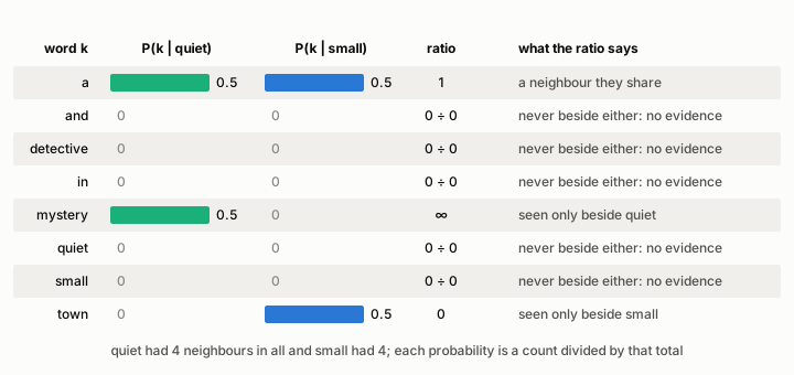 Figure 28.2. Neighbour probabilities of quiet and small from Figure 28.1. Their shared neighbour a gives a ratio of 1; mystery, seen only beside quiet, gives infinity; town, seen only beside small, gives 0.
The GloVe paper makes the same point with real numbers from a corpus of 6 billion tokens, reproduced in Figure 28.3. Take the target words ice and steam and a few probe words. “Solid” goes with ice far more than with steam, and the ratio of its two probabilities is 8.9. “Gas” goes with steam, and its ratio is 0.085. “Water” goes with both and “fashion” with neither, and their ratios sit near 1, at 1.36 and 0.96. The raw probabilities are tiny numbers that are hard to compare; the ratios sort the probe words cleanly into “about ice”, “about steam” and “about both or neither”.
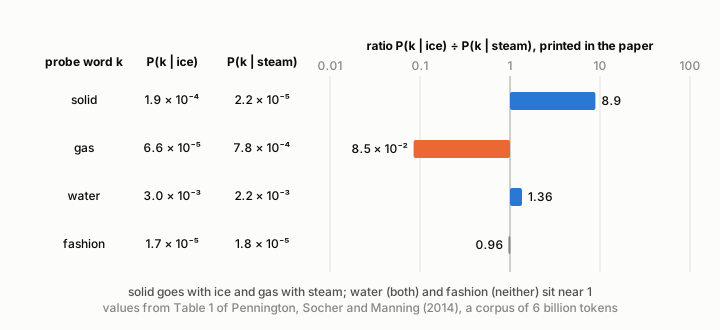 Figure 28.3. Table 1 of the GloVe paper, from a corpus of 6 billion tokens. The ratio of the two probabilities is 8.9 for solid and 0.085 for gas, and near 1 for water (1.36) and fashion (0.96). The printed ratios come from unrounded probabilities, so dividing the rounded ones does not reproduce them exactly.
From counts to vectors
GloVe then looks for two vectors per word, one for the word as a centre and one as a neighbour, such that the dot product of a centre vector and a neighbour vector, plus a small adjustment for each word, comes close to the logarithm of how often the two words occur together. A logarithm turns a ratio into a difference, so ratios of probabilities become differences between vectors, which is exactly the behaviour the ice and steam example asks for.
The fit is a weighted least-squares problem. With X for the co-occurrence counts, w for the vectors and b for the adjustments, GloVe makes this sum of squared errors as small as it can:
\[J = \sum_{i,j} f(X_{ij}) \left( w_i \cdot \tilde{w}_j + b_i + \tilde{b}_j - \log X_{ij} \right)^2\]Each error is multiplied by a weight f that depends on the pair’s count (Figure 28.4). Rare pairs, whose counts are noisy, get small weights. The weight grows as the count to the power 3/4 and stops growing at a count of 100, so that the commonest pairs cannot drown out the rest; the paper used exactly these values. The largest count in our tiny table, 2, would get a weight of only 0.05. The authors report that the vectors reached 75% accuracy on a test of word analogies.
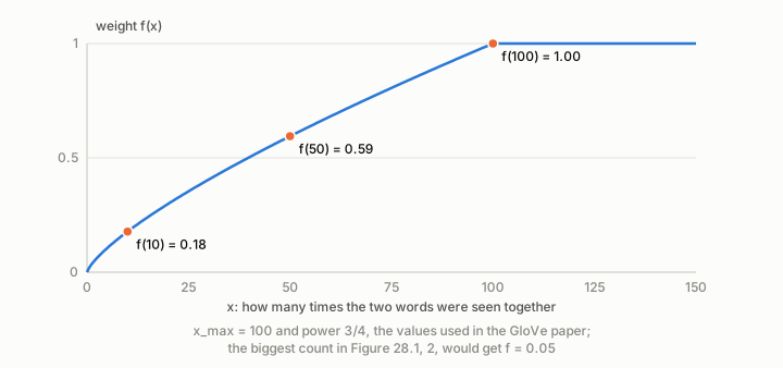 Figure 28.4. GloVe’s weight is (count ÷ 100) to the power 3/4, capped at 1: 0.18 for a count of 10, 0.59 for 50 and 1 from 100 on. The largest count in Figure 28.1, 2, would weigh 0.05.
Word2Vec and GloVe both produce static embeddings: one fixed vector per word, whatever sentence the word is in. The next chapter shows why that is not always enough.
Watch, read, try
- GloVe: Global Vectors for Word Representation (Stanford NLP) — the authors’ own summary, with downloadable pre-trained vectors.
Check yourself. 1. In Figure 28.1, what is P(small given town)? 2. Water and fashion both give ratios near 1. Why, when one is related to ice and steam and the other is not? 3. Why does GloVe stop the weight from growing beyond a count of 100?
Answers. 1. Town had 3 neighbours, two of them “small”, so 2 ÷ 3, about 0.67. 2. For water both probabilities are large and for fashion both are small; either way they are similar, so the ratio is close to 1. 3. So that very frequent pairs cannot dominate the fit.
29. Contextual embeddings and dimensionality reduction
In one breath. A static embedding gives a word one vector for life, but many words change meaning with their neighbours, so contextual models such as BERT compute a fresh vector for every use. Embeddings also tend to be long, and this chapter shows how to squeeze them: principal component analysis squeezes along straight lines, autoencoders along curves.
One word, two meanings
“Please book a table” and “the detective reads a book” use the same four letters for an action and for an object. A static table such as Word2Vec or GloVe looks up “book” by itself and returns the same row in both sentences (Figure 29.1, top). A contextual embedding is computed from the whole sentence, so the same word gets a different vector each time it is used (Figure 29.1, bottom). BERT, which chapter 32 describes, is the best-known model of this kind: it reads the whole input in both directions at once, and its output at each position depends on every word around it.
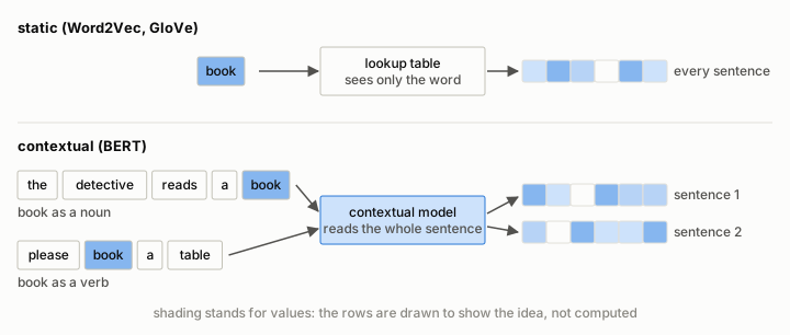 Figure 29.1. Static against contextual embeddings for “book” as a noun and as a verb. The shaded rows illustrate the idea; they are drawn, not computed.
Contextual models are usually pre-trained once, on a large amount of text with no labels, and then fine-tuned: training continues briefly on a smaller labelled data set for one task. BERT’s pre-training text came to about 3.3 billion words from books and from English Wikipedia.
Representation or embedding?
The two words overlap. In a 2022 answer on AI Stack Exchange, Edoardo Guerriero calls vector representation “a generic term” for any way of encoding data as numbers, and treats embeddings as a special case: continuous vectors of a fixed size, produced by a neural network or by factorising a matrix. In this book an embedding is always such a learned, fixed-size vector.
Squeezing along straight lines: PCA
Embeddings are often long, and long vectors are costly to store and hard to picture. Dimensionality reduction replaces each vector by a shorter one that keeps as much of the useful information as possible. The classic method is principal component analysis (PCA), invented by Karl Pearson in 1901. It finds the direction along which the points spread out most, then the direction of greatest spread at right angles to that one, and so on. These directions are the eigenvectors of the data’s covariance matrix, which is where chapter 6 pays off. Keeping only the first few directions keeps most of the spread with far fewer numbers.
Figure 29.2 uses the eight books of chapter 9, each a point with two numbers, pages and price. The two columns are measured in different units, so each is first standardised: its average is subtracted and the result divided by its standard deviation, which puts both on the same scale (chapter 14 explains why this matters). Pages and price rise together, with a correlation of 0.945, so the points lie close to one line. Projecting each book onto that line gives one number per book instead of two and keeps 97.3% of the total spread; the 2.7% lost is the grey drops. For two standardised columns the line always runs at 45 degrees, and its share of the spread is (1 + r) ÷ 2, where r is the correlation.
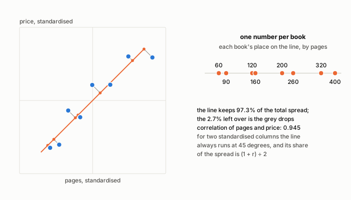 Figure 29.2. PCA on the eight books of chapter 9 after standardising both columns. Pages and price have correlation 0.945; the first direction keeps 97.3% of the spread, leaving 2.7% in the drops.
The same squeezing is often done with the singular value decomposition (SVD), which writes any table of numbers as a product of three simpler tables; its leading parts give the same directions as PCA, and PCA is often computed that way.
Squeezing along curves: autoencoders
An autoencoder is a neural network trained to copy its input to its output through a narrow middle layer called the code (Figure 29.3). The half before the code is the encoder and the half after it the decoder. Because the code holds fewer numbers than the input, the network cannot copy everything and must learn to keep what matters most. In their textbook, Goodfellow, Bengio and Courville show that with a straight-line decoder and squared error an autoencoder learns the same subspace as PCA, while a bent, non-linear encoder and decoder can follow curved structure that PCA would miss. They also warn that a network given too much freedom can learn to copy without learning anything useful.
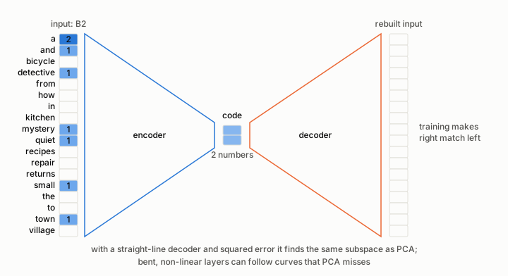 Figure 29.3. An autoencoder squeezes the 18 word counts of B2 into a code of 2 numbers and rebuilds them. The code and the rebuilt values are left blank: no network was trained for this picture.
From my notes. Two popular methods for dimensionality reduction are PCA and autoencoders: PCA is linear, autoencoders use neural networks for non-linear compression.
That is right, with one refinement from the paragraph above: an autoencoder whose layers are all straight lines can do no more than PCA, so the gain comes from the bends in its layers, not from being a neural network as such.
Watch, read, try
- What is the difference between representation and embedding? (AI Stack Exchange) — Edoardo Guerriero’s accepted answer, paraphrased in this chapter.
Check yourself. 1. Why does a static embedding give “book” the same vector in both sentences of Figure 29.1? 2. If pages and price had a correlation of 0 instead of 0.945, what share of the spread would the first PCA direction keep? 3. What goes wrong if an autoencoder’s code is as long as its input?
Answers. 1. It looks the word up in a table on its own; the rest of the sentence plays no part. 2. (1 + 0) ÷ 2, which is 50%: no direction is better than any other. 3. The network can learn to copy the input without learning anything useful; the narrow code is what forces it to choose.
Part VI: Sentences and attention
30. From the bottleneck to attention
In one breath. Early translation networks squeezed a whole sentence into one fixed-size vector before writing the translation, and long sentences suffered. Attention lets the writer look back at every input word at every step and choose where to look, which removed that bottleneck and became the core of modern language models.
Suppose a French customer asks what B1 says. “A quiet mystery in a small town” becomes “un mystère tranquille dans une petite ville”. Two things change on the way: the words, and in one place their order. French puts “tranquille” after its noun, while “petite” stays in front, as it does in English.
The encoder, the decoder and the bottleneck
In 2014 Ilya Sutskever, Oriol Vinyals and Quoc Le showed that a neural network could translate by reading the source sentence into a vector of fixed size and then writing the translation from that vector. The reader is the encoder and the writer the decoder. Both were recurrent networks, which take one word per step and carry a running summary forward from step to step (Figure 30.1). The summary handed from the encoder to the decoder is the context vector.
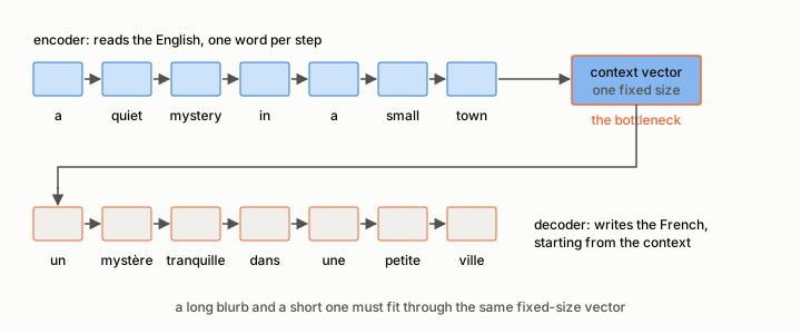 Figure 30.1. The encoder–decoder: B1 in English is read into one fixed-size context vector, from which the decoder writes “un mystère tranquille dans une petite ville”.
The trouble is the fixed size. Picture a clerk who reads a blurb aloud to a colleague who may write the translation only from notes kept on a single index card. A seven-word blurb fits on the card; a sixty-word review does not, and some of its detail has to go. Sutskever and his colleagues noticed a symptom of this: their system translated markedly better when it read each source sentence backwards, because the first source words then sat close to the first words the decoder had to write. In a paper first posted in 2014 and presented at ICLR in 2015, Dzmitry Bahdanau, Kyunghyun Cho and Yoshua Bengio suggested that this fixed-length vector was a bottleneck, and proposed a way round it.
Attention: a weighted look back
Keep every encoder state, not only the last. Bahdanau’s encoder read the sentence in both directions, so the state for each word summarised the whole sentence with the focus on that word’s surroundings; there is one such state per English word. At each decoder step, score how well each encoder state matches what the decoder needs at that moment, turn the scores into weights with softmax, and give the decoder the weighted sum of all the encoder states as its context for that step. Bahdanau and his colleagues computed the scores with a small learned network, and they described the effect in these words: “this implements a mechanism of attention in the decoder”. The decoder decides, step by step, which parts of the source to look at.
Figure 30.2 shows one step, the one that writes “tranquille”. The weight on “quiet” is 0.925, and the other six words share the remaining 0.075. Each of the seven states is multiplied by its weight and the results are added, so the context for this step is almost exactly the encoder’s state for “quiet”, which is what a translator needs at that moment. At the next step the weights are worked out afresh, and they move to “in”.
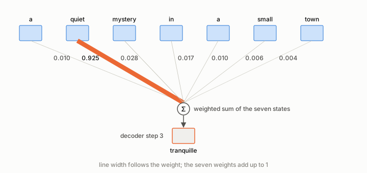 Figure 30.2. Attention for the decoder step that writes “tranquille”: weight 0.925 on quiet and 0.075 shared by the other six words. The weights come from the scoring rule of Figure 30.3.
The alignment map
Collect the weights of every decoder step into one table and you get an alignment map (Figure 30.3), with one row per French word and one column per English word. Most of the bright cells run down the diagonal, because the two languages keep most of their order; at “mystère” and “tranquille” the brightness crosses over. The weights here come from a made-up scoring rule, not from a trained model: 4 points when a French word translates an English word, minus half a point for each step of distance between their positions, then softmax along each row. The distance term matters for the two copies of “a”: “un” prefers the first (0.86 against 0.12) and “une” the second (0.85 against 0.12). The Bahdanau paper shows maps of this kind from its trained model, including a crossing where a French phrase reverses the order of the English adjectives. The map is also a gift to anyone who wants to check a model’s work: it shows, for every output word, which input words it drew on.
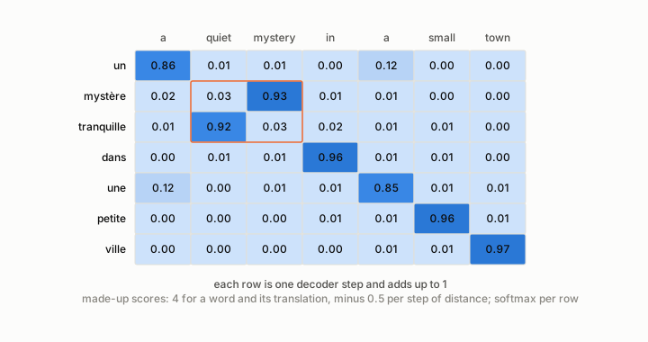 Figure 30.3. An alignment map from a made-up scoring rule (4 for a translation, minus 0.5 per step of distance, softmax per row). The swap at mystère and tranquille is the French adjective order; “un” and “une” each prefer the nearer “a” (0.86 and 0.85).
Looking back worked so well that in 2017 a team at Google asked whether the recurrent network was needed at all. Chapter 31 explains their answer, self-attention, and chapter 32 the model they built from it.
Watch, read, try
- NLP Course For You (Lena Voita) — the chapter “Seq2seq and Attention” is one of the clearest illustrated treatments of this material.
- Bahdanau, Cho and Bengio, Neural Machine Translation by Jointly Learning to Align and Translate — the paper that brought attention to translation.
- Foundations of Deep Learning (Hugo Larochelle), with the other eleven talks of the Deep Learning School of 24 and 25 September 2016: Deep Learning for Computer Vision (Andrej Karpathy), Deep Learning for Natural Language Processing (Richard Socher), TensorFlow Tutorial (Sherry Moore), Foundations of Unsupervised Deep Learning (Ruslan Salakhutdinov), Nuts and Bolts of Applying Deep Learning (Andrew Ng), Deep Reinforcement Learning (John Schulman), Theano Tutorial (Pascal Lamblin), Deep Learning for Speech Recognition (Adam Coates), Torch Tutorial (Alex Wiltschko), Sequence to Sequence Deep Learning (Quoc Le) and Foundations and Challenges of Deep Learning (Yoshua Bengio) — twelve introductory talks; Quoc Le’s covers the encoder–decoder of this chapter from one of its inventors.
Check yourself. 1. Why does a single context vector hurt long sentences more than short ones? 2. In Figure 30.2, why do the seven weights add up to exactly 1? 3. In Figure 30.3, why does “un” put some weight (0.12) on the second “a”?
Answers. 1. Everything must fit into the same fixed size, so a longer input has to be squeezed harder. 2. They come out of softmax, which always returns positive numbers that add up to 1. 3. Both copies of “a” match “un” equally well by meaning; only the distance penalty separates them.
31. Self-attention in plain words
In one breath. Self-attention lets every word of a sentence look at every other word of the same sentence and take a blend of them as its new vector. Three small steps do it (score, normalise, mix), and learned projections, several heads and position codes turn that idea into the engine of the transformer.
Three words, three steps
Take three words of B1 with this book’s two-number embeddings: quiet = (2, 0), mystery = (1, 1) and town = (0, 2), drawn on the left of Figure 31.1. Simple self-attention, as Peter Bloem teaches it in the lecture listed below, works in three steps.
First, score every pair of words by its dot product. Quiet against itself scores 2 × 2 + 0 × 0 = 4, quiet against mystery 2, and quiet against town 0. Second, turn each row of scores into weights with softmax, so that they are positive and add up to 1; quiet’s row (4, 2, 0) becomes 0.867, 0.117 and 0.016. Third, mix: each word’s output is the weighted sum of all the word vectors. For quiet that is 0.867 × (2, 0) + 0.117 × (1, 1) + 0.016 × (0, 2) = (1.851, 0.149).
Mystery’s scores are (2, 2, 2), so its weights are a third each and its output is (1, 1), mystery itself. The outputs are the hollow dots of Figure 31.1: quiet and town each lean a little towards the others, and mystery, already between them, stays where it was.
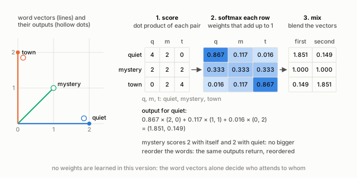 Figure 31.1. Simple self-attention on quiet (2, 0), mystery (1, 1) and town (0, 2). Quiet’s scores (4, 2, 0) become weights 0.867, 0.117 and 0.016, and its output is (1.851, 0.149). Mystery scores 2 with itself and 2 with quiet.
This version has no parameters at all, nothing that training could adjust. Who attends to whom is decided entirely by the word vectors, which is why Bloem stresses that whatever produces those vectors, typically an embedding layer, drives the attention.
Queries, keys and values
Real layers learn three matrices, which give each word three new descriptions: a query (what this word is looking for), a key (what this word offers to the queries of others) and a value (what this word hands on when it is chosen). Scores become query-against-key dot products, and the mix uses the values. Vaswani and his colleagues also divide every score by the square root of d, the number of entries in each query and key, because with many entries the dot products grow large and push softmax into regions where, in their words, “it has extremely small gradients”, which slows learning:
\[\text{Attention}(Q, K, V) = \text{softmax}\left( \frac{Q K^{\top}}{\sqrt{d}} \right) V\]Figure 31.2 picks the three matrices by hand to show what they can do: queries and values unchanged, keys with their two numbers swapped. Quiet’s query (2, 0) now matches town’s key best, so quiet puts 0.768 of its weight on town and only 0.045 on itself.
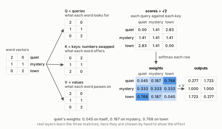 Figure 31.2. Queries against keys, scaled by the square root of 2. With the keys’ two numbers swapped, quiet puts 0.768 of its weight on town and 0.045 on itself.
Several heads
One set of weights captures one kind of relationship at a time. Multi-head attention runs several attention layers side by side, each with its own three matrices, and places their outputs next to each other before a final matrix mixes them. Figure 31.3 runs two heads on our three words. Head 1, with keys as they are, keeps each word mostly on itself; head 2, with swapped keys, pairs quiet with town. Joined, each word carries four numbers that describe two different views of the sentence. The original transformer used 8 heads of 64 numbers each, and because each head is small the total cost is about the same as one head of full width.
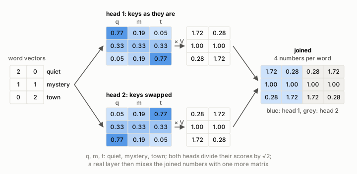 Figure 31.3. Two heads: head 1 (keys as they are) keeps each word mostly on itself, head 2 (keys swapped) pairs quiet with town. The joined outputs give each word four numbers.
Where am I? Position codes
Self-attention sees its input as a set, not a sequence. Reorder the three words of Figure 31.1 and the same three outputs come back, reordered in the same way; Bloem calls this property permutation equivariance. “The village returns to the detective” would look to it much like B4, the problem of Figure 26.4 in a new form. The cure is to add a position code to each word’s embedding before attention. The transformer paper uses waves: entry number 2i of the code for position pos is the sine of pos divided by 10000 raised to the power 2i ÷ d, and entry 2i + 1 is the cosine of the same angle.
Figure 31.4 draws a four-number code for the seven positions of B1. The first pair of entries turns quickly, the second pair slowly. The two copies of “a”, at positions 0 and 4, get different codes, (0, 1, 0, 1) and (−0.757, −0.654, 0.040, 0.999), so after the codes are added the two are no longer the same vector. The paper also tried position codes learned during training and found the results nearly identical.
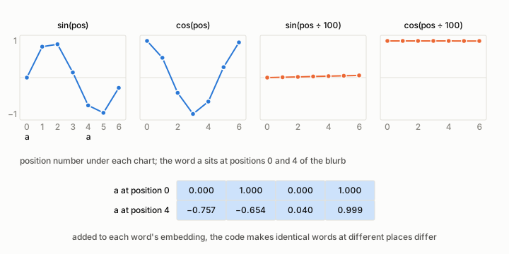 Figure 31.4. A four-number sinusoidal position code for the seven positions of B1. The two copies of “a” get (0, 1, 0, 1) at position 0 and (−0.757, −0.654, 0.040, 0.999) at position 4.
From my notes. Tip before watching the video: (1) think of the dot product as 3Blue1Brown’s projection of one vector onto another, so the dot product of a vector with itself is always larger than with any other vector; (2) input vectors are always converted into embeddings first, and it is the embedding that is fed into the model.
The note has the right instinct, and its second half is exactly right. The precise statement of the first half is this: among all vectors of the same length as A, the dot product with A is largest for A itself. Without the “same length” condition it fails. In Figure 31.1, mystery scores 2 with itself and also 2 with quiet, because quiet is longer; and a vector pointing the same way as mystery but twice as long, (2, 2), would score 4 with it, twice mystery’s own score. The reason is the rule behind the projection picture of chapter 4: a dot product equals the two lengths multiplied by the cosine of the angle between them, so a long vector can outscore a perfect match in direction. It is also why Bloem’s slide says a word’s weight on itself is usually the largest, not always.
Watch, read, try
- Lecture 12.1 Self-attention (Peter Bloem, DLVU) — simple self-attention first, then queries, keys, values and heads; the slide in my notes comes from this lecture.
- Intuition Behind Self-Attention Mechanism in Transformer Networks (Ark) — the score, normalise and weigh steps of this chapter, drawn for vectors of 50 numbers.
- Transformers from scratch (Peter Bloem) — the written companion to the lecture.
Check yourself. 1. What are mystery’s weights in Figure 31.1, and why? 2. Why do transformers divide the scores by the square root of d, the number of entries in each query and key? 3. Without position codes, how would self-attention treat “a small mystery in a quiet town” compared with B1?
Answers. 1. A third each: its three scores are all 2, and softmax of equal scores gives equal weights. 2. With many entries the dot products grow large, which pushes softmax towards all-or-nothing weights where learning slows. 3. Both use the same seven words, so it would return the same set of outputs, only reordered; it cannot tell the two blurbs apart.
32. Transformers and pretrained models
In one breath. In 2017 the transformer dropped recurrence altogether and built a translation model from attention, small feed-forward networks and a few simple devices. Its encoder half, trained once on billions of words and then adjusted for each task, became BERT and the family of pretrained models that followed.
The transformer block
Ashish Vaswani and seven colleagues at Google posted “Attention Is All You Need” in June 2017 and presented it at NIPS that year. Their encoder is a stack of identical blocks (Figure 32.1). Each block has two parts: multi-head self-attention from chapter 31, and a feed-forward network, two small layers applied to each word’s vector separately. Around each part runs a skip connection, which adds the part’s input back to its output, as in the residual networks of chapter 23, and after it comes layer normalisation, which shifts and rescales the numbers of each word’s vector to a standard average and spread before a learned adjustment. The original model stacked 6 blocks in the encoder and 6 in the decoder, with 512 numbers per word, 8 heads and a feed-forward layer 2,048 wide.
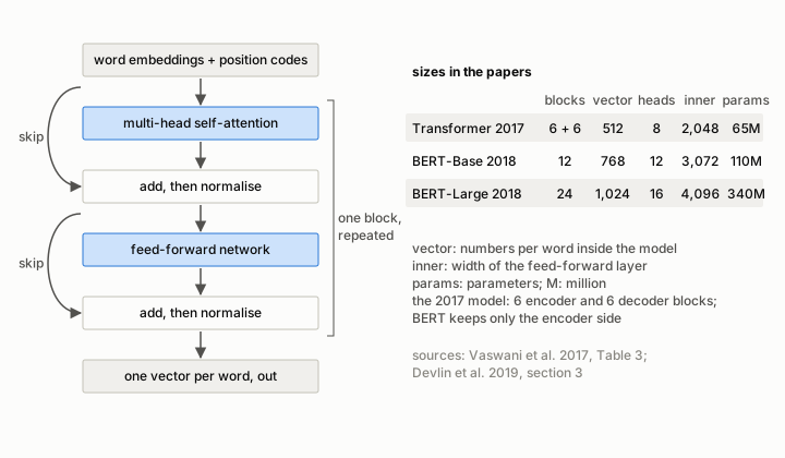 Figure 32.1. One transformer encoder block: self-attention and a feed-forward network, each followed by adding the input back and normalising. As published: 6 + 6 blocks and 512 numbers per word for the 2017 model; 12 and 24 blocks, 110 and 340 million parameters for BERT-Base and BERT-Large.
No step of a block waits for the previous word, so a transformer processes all the words of a sentence at once, which suits parallel hardware. The base model trained in 12 hours on 8 GPUs, and the larger version set a new best score on a standard English-to-German translation test.
BERT: pre-train once, fine-tune often
In October 2018 Jacob Devlin, Ming-Wei Chang, Kenton Lee and Kristina Toutanova at Google released BERT, which keeps only the encoder stack. They pre-trained it on two tasks that need no human labels (Figure 32.2, top). In the masked language model task, 15% of the input positions are chosen at random, most of them are replaced by a special [MASK] token, and the model must guess the original words from the context on both sides; in “a quiet [MASK] in a small town” the answer is “mystery”. Of the chosen positions, 80% get the mask, 10% a random word and 10% keep their own word, because the mask token never appears later, in fine-tuning. In next sentence prediction the model sees two passages and says whether the second really followed the first, which it did half the time. The text came from BooksCorpus (800 million words) and English Wikipedia (2,500 million words). The masked task is what makes BERT read in both directions. An earlier model, OpenAI’s GPT (Radford and colleagues, 2018), used a left-to-right design in which, as the BERT paper puts it, each token could attend only to the tokens before it.
BERT splits text into word pieces, frequent words whole and rare ones in fragments, from a vocabulary of 30,000. Every input begins with a special token, written [CLS], whose final vector stands for the whole input in classification tasks. The paper reports two sizes, below; a parameter is one adjustable number in the model, such as one entry of the embedding table or of a query matrix. In both sizes the feed-forward layer is four times as wide as the word vector, 3,072 and 4,096 numbers.
| Model | Blocks | Numbers per word | Heads | Parameters |
|---|---|---|---|---|
| BERT-Base | 12 | 768 | 12 | 110 million |
| BERT-Large | 24 | 1,024 | 16 | 340 million |
Fine-tuning (Figure 32.2, bottom) starts from the pre-trained weights, adds a small new part for the task, called a head, and trains everything briefly on labelled examples. The head here has two outputs and answers “is this blurb a mystery?” from the vector at [CLS]. The paper stresses that apart from the output layers the same network serves both stages, and that fine-tuning adjusts every parameter.
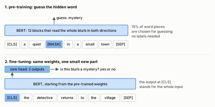 Figure 32.2. Pre-training fills in hidden words (15% of positions are chosen); fine-tuning adds a small head, here reading the output at the special first token.
Pre-training pays off most when labelled examples are scarce, which is the usual position of a small shop. In its study of model size, the BERT paper reports that the larger models were more accurate on all four tasks it tried, even one with only 3,600 labelled training examples.
BERT started a family. DistilBERT (2019) is 40% smaller and 60% faster while keeping 97% of BERT’s language understanding, by its authors’ measure. RoBERTa (2019) found that BERT had been significantly undertrained, and with longer, more careful training matched or beat the models published after it. ALBERT (2019) used two parameter-reduction techniques to cut memory use.
One thing BERT does not give you directly is a vector for a whole sentence: its output is one vector per word piece. The next chapter shows why the obvious fixes disappoint and what works instead.
Watch, read, try
- Vaswani et al., Attention Is All You Need — the transformer paper.
- Devlin et al., BERT: Pre-training of Deep Bidirectional Transformers for Language Understanding — the BERT paper, source of the sizes and pre-training details above.
Check yourself. 1. Why can a transformer process all the words of a sentence at once, while a recurrent encoder cannot? 2. In BERT’s masked language model, why is a chosen word not always replaced by [MASK]? 3. What does a skip connection add to a block’s output?
Answers. 1. No step depends on the output of the previous step; attention looks at all positions together. 2. The [MASK] token never appears during fine-tuning, so mixing in random and unchanged words narrows the gap between the two stages. 3. The block’s own input, so the block only has to learn a correction to it.
33. Sentence embeddings and sentence transformers
In one breath. To find similar blurbs among thousands you need one vector per blurb, computed once and compared cheaply. Sentence-BERT fine-tunes BERT so that its averaged word vectors become good sentence vectors, cutting the search for the closest pair among 10,000 sentences from about 65 hours to about 5 seconds.
Two ways to compare sentences
BERT can judge how alike two sentences are if you feed it both at once, joined by a separator token: this arrangement is a cross-encoder (Figure 33.1, left). It is accurate, but every pair needs its own pass through the network. Nils Reimers and Iryna Gurevych worked out the cost in their 2019 paper. With n sentences there are n × (n − 1) ÷ 2 pairs, so finding the most similar pair among 10,000 sentences takes 49,995,000 passes, about 65 hours on a V100 GPU. The shop’s five blurbs make only 10 pairs; a catalogue of ten thousand is another matter.
A bi-encoder (Figure 33.1, right) runs each sentence through the network once, keeps the resulting vector and compares vectors by cosine similarity. For the same 10,000 sentences that costs about 5 seconds of encoding and about 0.01 seconds of cosines (Figure 33.2).
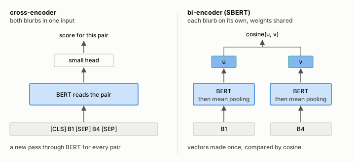 Figure 33.1. A cross-encoder reads each pair together; a bi-encoder (SBERT) turns each blurb into a vector once and compares vectors.
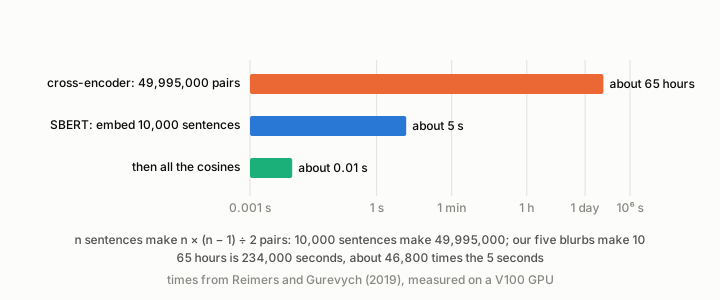 Figure 33.2. The SBERT paper’s costs for 10,000 sentences: 49,995,000 pairs through a cross-encoder take about 65 hours (234,000 seconds, about 46,800 times the 5 seconds SBERT needs to embed them). Times as measured by the authors on a V100 GPU.
Pooling and Sentence-BERT
BERT’s output holds one vector per word piece, so a sentence vector needs pooling, some way of combining the word vectors into one. Mean pooling averages them; max pooling keeps the largest value in each position; CLS pooling takes the vector of the first, special token. The obvious approach, pooling the outputs of plain BERT, works poorly. On seven tests that compare a model’s similarity scores with human ratings, the paper reports 54.81 for averaged BERT vectors and 29.19 for the CLS vector, both below the 61.32 of averaged GloVe vectors (the scores are rank correlations with the human ratings, multiplied by 100).
SBERT fine-tunes BERT so that pooled vectors become useful. It uses a siamese network: one encoder, with one set of weights, applied to each sentence of a pair (Figure 33.3). The training pairs come from natural language inference, the task of deciding whether one sentence follows from another (entailment), contradicts it (contradiction) or neither (neutral). The data were SNLI, with 570,000 labelled sentence pairs, and MultiNLI, with 430,000. For each pair, the two mean-pooled vectors u and v are joined with their element-wise difference |u − v|, and a small classifier predicts one of the three labels with softmax and a cross-entropy loss. Training made a single pass over the data.
In Figure 33.3 the encoder is the made-up feature table of chapter 25, so every number can be checked: u = (0.20, 0.24, 0.03, 0.01) for B1, v = (0.20, 0.18, 0.05, 0.05) for B4, and their difference is (0.00, 0.06, 0.02, 0.04). After training the classifier is thrown away; only the encoder is kept, and sentences are compared by cosine.
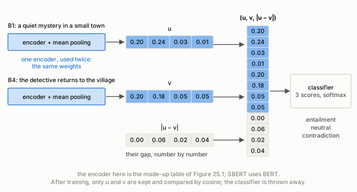 Figure 33.3. SBERT’s training path with the made-up table of chapter 25 as the encoder: u = (0.20, 0.24, 0.03, 0.01), v = (0.20, 0.18, 0.05, 0.05), and their element-wise difference (0.00, 0.06, 0.02, 0.04).
The paper’s ablation study, which changes one ingredient at a time, shows which choices matter. After NLI training, mean pooling, the paper’s default, scored 80.78, the CLS vector 79.80 and max pooling 79.07. The join mattered much more: u and v alone scored 66.04, while u, v and |u − v| together scored 80.78, and the authors single out the element-wise difference as the most important part. On the seven similarity tests, SBERT built on BERT-Base averaged 74.89, against 54.81 for averaged plain BERT.
What sentence vectors buy you
Figure 33.4 compares the five blurbs in two ways. Counted words say that B1 and B4 have nothing in common, a cosine of 0. Averaged word vectors, even the crude made-up ones of chapter 25, put them at 0.98, because both are about crime in a small place, while the bicycle blurb stays apart at 0.09. With only four made-up features the three crime blurbs look almost identical; real models with hundreds of learned numbers separate finer shades. That is the promise of sentence embeddings: search by meaning rather than by shared words.
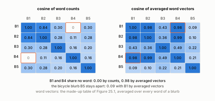 Figure 33.4. B1 and B4 share no word: cosine 0 by counts, 0.98 by averaged made-up word vectors. The bicycle blurb B5 stays at 0.09 from B1.
Newer sentence transformers
Since 2019 many models have been trained on the same plan with more data and better losses. The sentence-transformers documentation now leads with general-purpose models trained on more than a billion sentence pairs, and its notes on NLI training say the loss of the original paper does not give the best results. A multiple negatives ranking loss does better: each sentence must pick its true partner out of all the other sentences in the training batch. The original SBERT model no longer appears in the documentation’s table. Four of its entries, as read on 28 September 2026, are below; the sentence score averages 14 sentence tasks, the search score 6 search tasks, and speed is sentences encoded per second on a V100 GPU.
| Model | Sentence score | Search score | Speed | Size (MB) | Numbers per text |
|---|---|---|---|---|---|
| all-mpnet-base-v2 | 69.57 | 57.02 | 2,800 | 420 | 768 |
| all-MiniLM-L6-v2 | 68.06 | 49.54 | 14,200 | 80 | 384 |
| all-roberta-large-v1 | 70.23 | 53.05 | 800 | 1,360 | 1,024 |
| averaged GloVe vectors | 49.79 | 22.71 | 34,000 | 420 | 300 |
The documentation names all-mpnet-base-v2 as the best in quality, and says all-MiniLM-L6-v2 is five times faster while still offering good quality. Two further ideas from the reading list refine the picture. Matryoshka embeddings, after Kusupati and colleagues (2022), are trained so that the first numbers of a vector work on their own, which lets you cut a vector short to save space and time. ColBERT, from Omar Khattab and Matei Zaharia (2020), keeps one vector per word piece and compares a query with a document word piece by word piece, a “late interaction” that stays cheaper than a cross-encoder.
Watch, read, try
- Reimers and Gurevych, Sentence-BERT: Sentence Embeddings using Siamese BERT-Networks — the paper; the numbers in this chapter come from its sections 1, 3, 4, 6 and 7.
- Sentence Transformers: Meanings in Disguise (Pinecone) — James Briggs’s walk-through from attention to SBERT and its successors.
- Intro to Sentence Embeddings with Transformers (James Briggs) — the video version of the same walk-through.
- Pretrained models (sbert.net) — the current table of models; the link now forwards to the documentation’s new address.
- Natural Language Inference, current page (sbert.net) — where those training notes now live, with the softmax and multiple negatives ranking losses.
- MPNet (Hugging Face documentation) — the model behind all-mpnet-base-v2; the link forwards to the current documentation.
- Sentence Embeddings (Hugging Face Space by flax-sentence-embeddings) — an interactive app for trying sentence-embedding models in the browser.
- Introduction to Matryoshka embedding models (Hugging Face) — vectors you can cut short.
- ColBERT: a complete guide (Medium) — one vector per word piece and late interaction.
- Customizing reusable frozen ML-embeddings with Vespa — keep one set of document vectors and adapt only the query side for each task.
Check yourself. 1. How many passes would a cross-encoder need to compare every pair among 100 blurbs? 2. Why is |u − v| useful to SBERT’s classifier? 3. How can B1 and B4 score 0.98 with averaged word vectors but 0 with counts?
Answers. 1. 100 × 99 ÷ 2 = 4,950. 2. It shows, number by number, where the two sentence vectors differ; the paper’s ablation found it the most important part of the join. 3. Counts need shared words, and the two blurbs share none; word vectors let different words with related meanings contribute similar numbers.
Appendix
A. Where each note went
Each of the eleven note files became one or more chapters. Nothing was carried over unread; the reasons for leaving out a screenshot or a paragraph were recorded during the rewrite.
| Note file | What it held | Where it went |
|---|---|---|
| linearAlgebra.docx | 3Blue1Brown frames and reminders on dot products, cross products, Cramer’s rule, change of basis and eigenvectors | chapters 1 to 6 |
| matrixmultiplication.xyz.docx | two screenshots of an interactive matrix-multiplication page | chapter 2 |
| neuralNetworks.docx | a reminder about ReLU and a slide on non-linear activations | chapter 7 |
| backPropGrads.docx | three video links and a computation-graph slide | chapter 8 |
| biasAndVariance.docx | forty StatQuest frames on bias, variance, cross-validation and ridge regression | chapters 9 to 11 |
| Untitled document.docx | a pasted article on identifying the distribution of a sample | chapter 13 |
| feraturesAndEngineering.docx | links and fragments on categorical columns, scaling, quantile normalisation, batch normalisation and PMF, PDF and CDF | chapters 12, 14, 15, 16 |
| cnn.docx | reminders, a long link list, three pasted articles on convolutional networks, and self-attention frames | chapters 17 to 24 and 31 |
| filtersAndKernels.docx | an excerpt on filters as collections of kernels | chapter 18 |
| embedding.docx | two pasted guides on word embeddings and a page on embedding models | chapters 25 to 29 |
| embedding_sentence.docx | a pasted article on sentence transformers | chapters 30, 32, 33 |
B. Glossary
- 1 × 1 convolution — a convolution that mixes the channels at each pixel without looking at its neighbours (chapter 22).
- activation function — the bend applied to a neuron’s weighted sum, such as ReLU, which replaces negative values by zero (chapter 7).
- adversarial example — an input changed very slightly on purpose so that a model misclassifies it (chapter 23).
- alignment map — a table of attention weights with one row per output word and one column per input word, showing which input words each output word drew on (chapter 30).
- Anderson–Darling test — a goodness-of-fit test that compares a sample’s staircase CDF with a fitted CDF, weighting the tails heavily (chapter 13).
- attention — a mechanism that gives a network, at each step, a weighted sum of many stored vectors, with weights computed from how well each vector matches the current need (chapter 30).
- autoencoder — a neural network trained to rebuild its input from a narrower middle layer, the code, so that the code must keep what matters most (chapter 29).
- average pooling — pooling that keeps the mean of each window (chapter 20).
- backpropagation — computing every gradient of a network in one backward sweep with the chain rule, reusing products along the way (chapter 8).
- backward pass — running a computation graph from the output back to the inputs to collect every gradient (chapter 8).
- bagging — fitting a model to each of many resampled copies of the data and averaging them to reduce variance (chapter 9).
- bag of words — a text written as the count of each vocabulary word in it, ignoring word order (chapter 26).
- basis — a set of vectors whose linear combinations reach every point of the space in exactly one way (chapters 1 and 5).
- batch normalisation — standardising a unit’s weighted sums over a mini-batch, then applying a learned scale γ and shift β (chapter 16).
- BERT — a pre-trained stack of transformer encoder blocks that reads text in both directions and returns one contextual vector per word piece (chapter 32).
- bias (of a filter) — the single number a filter adds to every cell of its output map (chapter 18).
- bias (of a model) — the systematic error of a model: how far its average prediction is from the truth, typically large for models too simple for the data (chapter 9).
- bias (of a neuron) — the number a neuron adds to its weighted sum whatever the inputs are; not the same as a model’s bias (chapter 7).
- bias–variance trade-off — more flexibility lowers bias and raises variance, so test error is lowest somewhere in between (chapter 9).
- bi-encoder — a model that turns each sentence into its own vector once, so that sentences are compared by a cheap similarity such as the cosine (chapter 33).
- boosting — fitting models one after another, each to the errors the earlier ones left (chapter 9).
- bottleneck — in an encoder–decoder, the single fixed-size context vector through which all information about the input must pass (chapter 30).
- bottleneck block — a residual block that narrows the channels with a 1 × 1 convolution before its 3 × 3 and widens them after (chapter 22).
- categorical column — a column of labels that sort items into groups, even if the labels are digits (chapter 14).
- Cauchy product — the rule that a product of polynomials has the convolution of their coefficient lists as its coefficients (chapter 24).
- Cauchy–Schwarz inequality — a dot product never exceeds the product of the two vectors’ lengths (chapter 4).
- CBOW (continuous bag of words) — the Word2Vec game that averages the vectors of a word’s neighbours and trains them to predict the word (chapter 27).
- chain rule — the slope along a chain of steps is the product of the steps’ slopes (chapter 8).
- change of basis — translating a vector’s coordinates from one basis to another, by the matrix whose columns are the new basis vectors or by its inverse (chapter 5).
- channel — one layer of values stacked over the same grid of positions, such as the red, green or blue plane of a colour image (chapters 17 and 18).
- characteristic polynomial — det(M − λI) written out as a polynomial in λ, whose roots are the eigenvalues (chapter 6).
- class-specific quantile normalisation — quantile normalisation applied separately within each class, preserving differences between classes (chapter 15).
- CLS token — the special first token of every BERT input, whose final vector stands for the whole input in classification tasks (chapter 32).
- code — the narrow middle layer of an autoencoder, the compressed version of the input (chapter 29).
- ColBERT — a retrieval model that keeps one vector per word piece and compares query and document word piece by word piece, a late interaction (chapter 33).
- commutative — describes an operation whose answer does not change when its two inputs swap places, which matrix multiplication is not (chapter 2).
- computation graph — a calculation drawn as boxes, each taking a few numbers and returning one, joined by arrows (chapter 8).
- contextual embedding — a word vector computed from the whole sentence, so the same word gets a different vector in each use (chapter 29).
- context vector — the vector an encoder hands to a decoder; one fixed vector in the plain encoder–decoder, a fresh weighted sum at every step with attention (chapter 30).
- context window — the few words on each side of a centre word that count as its neighbours (chapter 27).
- continuous — a quantity that can take any value in a range, such as a length (chapter 12).
- convolution (in deep learning) — sliding a kernel over a grid, multiplying cell by cell and adding at each position; strictly a cross-correlation (chapter 17).
- convolution of distributions — the distribution of a sum of two independent quantities, found by multiplying and adding matching pairs of probabilities (chapter 24).
- co-occurrence matrix — a table counting how often each word appears within a window of each other word across a whole corpus (chapter 28).
- coordinate — one of the numbers in a vector, saying how far it goes along one axis (chapter 1).
- cosine similarity — the dot product of two vectors divided by the product of their lengths: 1 for the same direction, 0 at a right angle, −1 for opposite (chapters 25 and 27).
- Cramer’s rule — a way to solve a small system of linear equations by replacing one column of the matrix with the output and dividing determinants (chapter 3).
- cross-correlation — convolution without flipping the kernel, which is what deep-learning libraries compute (chapter 17).
- cross-encoder — a model that reads two sentences together and returns one score for the pair, accurate but needing a pass for every pair (chapter 33).
- cross-entropy loss — the training penalty for a classifier: minus the logarithm of the probability it gave to the correct answer, small when it was confident and right and large when it was confident and wrong (chapter 33).
- cross product — for two vectors in three dimensions, the vector perpendicular to both whose length is the area of their parallelogram (chapter 4).
- cross-validation — estimating how well a model generalises by training on some blocks of the data and testing on the block held out, in turn (chapter 10).
- cumulative distribution function (CDF) — the probability that a quantity is at most a given value, a running total or area from the left (chapter 12).
- decoder — the part of a network that turns a compact representation back into a full output: the second half of an autoencoder, or the writer of a translation (chapters 29 and 30).
- dense layer — a layer in which every output is a weighted sum of every input (chapter 19).
- dense vector — a short vector with mostly non-zero entries (chapter 25).
- density — probability per unit of the measured quantity; a height on a PDF, not itself a probability (chapter 12).
- depthwise separable convolution — a depthwise step, one kernel per channel, followed by a pointwise 1 × 1 step that mixes channels (chapter 22).
- derivative — the rate at which an output changes per unit change of one input, for very small changes (chapter 8).
- determinant — the factor by which a matrix scales every area or volume, negative when the move flips space over (chapter 3).
- diagonalisable matrix — a matrix with enough eigenvectors for an eigenbasis, in which it becomes diagonal (chapter 6).
- diagonal matrix — a matrix whose entries off the main diagonal are all zero, so it only stretches along the axes (chapter 6).
- dilated convolution — a convolution whose kernel taps are spread apart with gaps, widening its reach without more weights (chapter 22).
- dimension — how many numbers a vector has, or how many axes a space has (chapter 1).
- dimensionality reduction — describing each item with fewer numbers than it came with, for example by projecting onto the few directions along which the data varies most (chapters 4 and 29).
- discrete — a quantity that can take only separate, countable values, such as the number of books bought (chapter 12).
- document frequency — the number of texts in a collection that contain a given word at least once (chapter 26).
- dot product — the sum of the products of matching entries of two vectors, equal to the product of their lengths and the cosine of the angle between them (chapter 4).
- duality — the correspondence between a 1 × n matrix, which turns vectors into numbers, and the vector whose dot product does the same job (chapter 4).
- effective receptive field — the Gaussian-shaped central part of a receptive field that actually carries most of the influence (chapter 21).
- eigenbasis — a basis made entirely of eigenvectors of a matrix (chapter 6).
- eigenvalue — the factor by which a matrix stretches one of its eigenvectors; negative when the vector is turned round (chapter 6).
- eigenvector — a vector that a transformation keeps on its own line, only stretching it by a factor called the eigenvalue (chapter 6).
- embedding — a dense, usually learned vector of fixed length that stands for an object, arranged so that similar objects get similar vectors (chapter 25).
- embedding layer — a table with one row per vocabulary word; embedding a word means reading its row, which equals multiplying its one-hot code by the table (chapter 25).
- embedding model — a model that turns an object of any size, such as a text, into a vector of one fixed length (chapter 25).
- encoder — the part of a network that reads an input and turns it into a compact representation: the first half of an autoencoder, or the reader of a sentence to be translated (chapters 29 and 30).
- ensemble — several trained models whose predictions are combined (chapter 23).
- entailment — in natural language inference, the label for a pair where the second sentence follows from the first (chapter 33).
- equivariant — shifting the input shifts the output by the same amount (chapter 20).
- fat-pencil test — the informal check that a probability plot’s dots would be hidden by a fat pencil laid along the line (chapter 13).
- feature — one column of the table a model learns from (chapter 14).
- feature detector — an informal name for a filter, after what it does (chapter 18).
- feature engineering — turning raw columns into features a model can use well (chapter 14).
- feature map — an output channel of a convolution, showing where the filter’s pattern appears (chapter 17).
- feature visualisation — adjusting an image, starting from noise, until a chosen unit responds strongly, to see what the unit looks for (chapter 19).
- feed-forward network — in a transformer block, two small layers applied to each word’s vector separately (chapter 32).
- filter — with several input channels, the stack of kernels (one per input channel) whose results are summed with one bias to give one output channel (chapter 18).
- fine-tuning — continuing to train a pre-trained model briefly on a smaller labelled data set for one task (chapters 29 and 32).
- flip and slide — reading one list backwards and shifting it along the other to line up the pairs a convolution multiplies (chapter 24).
- fold — one of the blocks the data are split into for cross-validation (chapter 10).
- forward pass — running a computation graph from its inputs to its output (chapter 8).
- gamma distribution — a right-skewed two-parameter family often used for positive measurements (chapter 13).
- Gaussian elimination — solving linear equations by subtracting multiples of one equation from another until the unknowns come out one at a time (chapter 3).
- global average pooling — averaging each whole channel into a single number, usually at the end of a network (chapter 20).
- GloVe — a method that learns word vectors whose dot products match the logarithms of co-occurrence counts, weighted so that rare and very frequent pairs do not dominate (chapter 28).
- goodness-of-fit test — a test of whether a sample could have come from a stated distribution; a high p-value keeps the distribution as a candidate (chapter 13).
- gradient — the collection of an output’s slopes with respect to each input, one number per input (chapter 8).
- gradient descent — the training loop that moves every weight a small step against its gradient and repeats until the error stops falling (chapters 8 and 14).
- head (attention) — one of several attention layers run side by side, each with its own query, key and value matrices (chapter 31).
- head (task) — a small new part added on top of a pre-trained model for one task, such as a two-way classifier (chapter 32).
- hidden layer — a layer between a network’s inputs and its output (chapter 7).
- hierarchical softmax — a shortcut for scoring a large vocabulary by arranging the words in a binary tree, used in the first Word2Vec paper (chapter 27).
- identity matrix — the do-nothing matrix, with ones on its diagonal and zeros elsewhere, written I (chapter 6).
- imaginary unit — the number i whose square is −1; a quarter turn’s eigenvalues are i and −i (chapter 6).
- imbalanced classes — a target in which one class is much rarer than the others, making accuracy misleading (chapter 14).
- intercept — the height at which a line crosses the vertical axis; ridge regression does not penalise it (chapter 11).
- internal covariate shift — Ioffe and Szegedy’s name for the changing distribution of a layer’s inputs during training (chapter 16).
- interquartile range (IQR) — the distance between the 25th and 75th percentiles (chapter 14).
- invariant — shifting the input leaves the output unchanged (chapter 20).
- inverse document frequency (idf) — the logarithm of the number of texts divided by the number that contain the word; large for rare words (chapter 26).
- inverse matrix — the matrix that undoes a transformation, which exists exactly when the determinant is not zero (chapter 3).
- IQR rule — flagging values more than 1.5 interquartile ranges beyond the quartiles (chapter 14).
- jump — the distance in input pixels between neighbouring units of a layer, the product of the strides before it (chapter 21).
- kernel — a small grid of weights that slides over an image, multiplying and adding at each position (chapters 17 and 18).
- key — the description of a word that is matched against the queries of other words in attention (chapter 31).
- lasso — a relative of ridge regression whose penalty uses the slopes’ sizes instead of their squares, and which can set some slopes exactly to zero (chapter 11).
- layer — a set of neurons that read the same inputs, computing a matrix times a vector plus a vector and then an activation (chapter 7).
- layer normalisation — rescaling the numbers of each word’s vector to a standard average and spread, followed by a learned adjustment (chapter 32).
- least squares — choosing the line or curve whose squared misses add up to the smallest total (chapter 9).
- leave-one-out cross-validation — cross-validation in which each round holds back a single data point (chapter 10).
- likelihood-ratio test (LRT P) — a test of whether a third parameter improves a fit enough to keep it (chapter 13).
- linear combination — a sum of scaled vectors, such as 3î + 2ĵ (chapter 1).
- linear transformation — a way of moving every point that keeps the origin fixed and grid lines straight, parallel and evenly spaced (chapter 2).
- local outlier factor — a score that flags rows lying in much emptier space than their neighbours (chapter 14).
- logistic regression — a single weighted sum passed through a sigmoid to give a probability (chapter 7).
- lognormal distribution — the distribution of a quantity whose logarithm follows a normal curve; skewed to the right (chapter 12).
- log transform — replacing values by their logarithms so that each factor of ten becomes one equal step (chapter 14).
- masked language model — BERT’s pre-training task of guessing words hidden in the input from the context on both sides (chapter 32).
- matrix — a grid of numbers whose columns say where the basis arrows land, so that multiplying by it transforms the whole grid (chapter 2).
- matrix product — the matrix of doing one transformation after another, written with the first move on the right (chapter 2).
- Matryoshka embedding — an embedding trained so that its first numbers work on their own, letting the vector be cut short (chapter 33).
- max pooling — pooling that keeps the largest value in each window (chapter 20).
- mean pooling — making one sentence vector by averaging the vectors of its word pieces (chapter 33).
- mean squared error — the average of the squared differences between predictions and true values (chapter 9).
- mini-batch — the small group of training examples used for one step of gradient descent (chapter 16).
- min–max scaling — rescaling a column so its smallest value becomes 0 and its largest 1 (chapter 14).
- mixture — a blend of two or more distributions in one sample (chapter 13).
- multi-head attention — several attention heads run side by side, their outputs placed next to each other and mixed by one more matrix (chapter 31).
- multiple negatives ranking loss — a training loss that asks each sentence to pick its true partner out of all the other sentences in the batch (chapter 33).
- natural language inference — deciding whether one sentence follows from another, contradicts it, or neither (chapter 33).
- negative sampling — training Word2Vec to tell a true neighbour from a few randomly drawn noise words instead of scoring the whole vocabulary (chapter 27).
- neuron — a unit that multiplies each input by a weight, adds a bias and passes the total through an activation function (chapter 7).
- next sentence prediction — BERT’s second pre-training task: saying whether one passage really followed another (chapter 32).
- one-hot encoding — writing a word as a row of zeros with a single 1 in the word’s own column (chapter 25).
- ordered category — a categorical column whose labels have a natural order, such as book condition (chapter 14).
- origin — the point (0, 0) where the axes cross and every vector-arrow starts (chapter 1).
- orthogonal matrix — a matrix whose columns are perpendicular vectors of length one, which keeps every length, angle and dot product; also called orthonormal (chapter 4).
- outlier — a value far from the rest of its column (chapter 14).
- overfitting — fitting the training data so closely that a less flexible model would have done better on new data (chapter 9).
- padding — a border of zeros added around an input before convolving, so that edges get their turn at a window’s centre (chapter 17).
- parallelepiped — a slanted box whose six faces are parallelograms (chapters 3 and 4).
- parameter — one adjustable number in a model, such as an entry of a weight matrix (chapter 32).
- parameter sharing — using the same weights at every position of the input (chapter 19).
- parsimony — preferring the simplest description that fits the data well enough (chapter 13).
- percentile — a quantile written as a percentage, such as the 25th percentile for the 0.25 quantile (chapter 12).
- permutation equivariance — the property that reordering the inputs reorders the outputs in the same way and changes nothing else; plain self-attention has it (chapter 31).
- pixel — one cell of an image’s grid of numbers (chapter 17).
- polynomial degree — the highest power in a polynomial; each extra degree allows one more bend (chapter 9).
- pooling (in images) — summarising each small window of a feature map by its maximum or average (chapter 20).
- pooling (of word vectors) — combining the vectors of a sentence’s word pieces into one sentence vector: mean, max or CLS (chapter 33).
- position code — a vector added to each word’s embedding that tells attention where in the sentence the word stands (chapter 31).
- pre-training — training a model once on a large amount of unlabelled text before adapting it to tasks (chapters 29 and 32).
- principal component analysis (PCA) — finding the directions along which data spread most, the eigenvectors of the covariance matrix, and keeping only the first few (chapter 29).
- probability density function (PDF) — a curve for a continuous quantity whose area between two values is the probability of landing between them (chapter 12).
- probability mass function (PMF) — the list of probabilities of each possible value of a discrete quantity, adding up to 1 (chapter 12).
- probability plot (Q–Q plot) — a plot of a sample’s sorted values against a fitted model’s quantiles; a straight line means a good fit (chapter 13).
- probability ratio — in GloVe, P(k given i) divided by P(k given j), large or small for words tied to one target and near 1 for words tied to both or neither (chapter 28).
- projection — the point reached by dropping straight onto a line, and its distance from the origin along that line; the book calls it a shadow (chapter 1).
- qsmooth — a variant of quantile normalisation that weighs differences between groups against variation within them (chapter 15).
- quantile — the value below which a chosen fraction of a distribution or sample falls; the median is the 0.5 quantile (chapter 12).
- quantile normalisation — making several samples share one distribution by giving equal ranks equal values (chapter 15).
- query — the description of what a word is looking for, matched against the keys of all words in attention (chapter 31).
- rank mean — the average, across samples, of the values at one rank; the shared value quantile normalisation assigns to that rank (chapter 15).
- receptive field — the region of the original input that can change one unit’s value (chapter 21).
- recurrent network — a network that takes one input per step and carries a running summary from step to step (chapter 30).
- regularisation — charging a model for complexity so that it prefers simpler fits (chapters 9 and 11).
- ReLU — the rectified linear unit, which returns its input when positive and 0 otherwise (chapter 7).
- residual block — a block that outputs F(x) + x, so its layers learn the change to make (chapter 23).
- ridge regression — least squares with a penalty on the squared size of the coefficients, which trades a little bias for less variance (chapter 11).
- right-hand rule — curl the right hand’s fingers from the first vector to the second and the thumb gives the cross product’s direction (chapter 4).
- robust scaling — subtracting the median and dividing by the interquartile range, which outliers barely move (chapter 14).
- scaled dot-product attention — attention whose scores are query–key dot products divided by the square root of the vector length before softmax (chapter 31).
- scaling — multiplying a vector by a number, which stretches it or, for a negative number, flips it (chapter 1).
- self-attention — attention in which every word of a sentence scores every other word of the same sentence and takes a weighted blend of them (chapter 31).
- semantic search — finding texts by meaning rather than by shared words, usually by comparing embeddings (chapters 25 and 33).
- Sentence-BERT (SBERT) — BERT fine-tuned in a siamese network on sentence pairs so that its mean-pooled vectors can be compared by cosine (chapter 33).
- sentence embedding — one vector for a whole sentence or text, fixed in length (chapter 33).
- siamese network — one encoder with one set of weights applied to each item of a pair (chapter 33).
- sigmoid — an S-shaped activation whose outputs lie between 0 and 1, the function used by logistic regression (chapter 7).
- similar matrices — two matrices related by A⁻¹MA that describe the same transformation in two different bases (chapter 5).
- singular value decomposition (SVD) — writing any table of numbers as a product of three simpler tables; its leading parts give the principal directions (chapter 29).
- skew — lopsidedness of a distribution; a right skew has a long tail towards large values (chapter 13).
- skip connection — adding a block’s input to its output, so the block learns a correction; also called a residual connection (chapters 23 and 32).
- skip-gram — the Word2Vec game that uses a word’s vector to predict each of its neighbours (chapter 27).
- Sobel kernel — a hand-made 3 × 3 kernel that measures left-to-right change and so finds vertical edges (chapter 19).
- softmax — turning a list of scores into positive weights that add up to 1 by exponentiating each score and dividing by the total (chapters 27 and 31).
- span — for one non-zero vector, the line through the origin made of all its multiples; in general, all the combinations of a set of vectors (chapter 6).
- sparse interactions — each output of a convolution depending on only a few inputs (chapter 19).
- sparse vector — a vector whose entries are almost all zero, such as a one-hot code or a bag of words (chapters 25 and 26).
- spatially separable kernel — a kernel that equals a column times a row, so it can be applied as two cheaper passes (chapter 22).
- squeeze-and-excitation (SE) — a block that averages each channel, turns the averages into gates with two small layers and a sigmoid, and rescales each channel by its gate (chapter 23).
- standard error (of an average) — the standard deviation of some scores divided by the square root of how many there are, a measure of how much their average could move (chapter 10).
- standardisation (z-score) — subtracting a column’s mean and dividing by its standard deviation (chapter 14).
- standardise — subtract a column’s average and divide by its standard deviation, putting columns in different units on one scale (chapters 14 and 29).
- static embedding — one fixed vector per word, whatever sentence it appears in, as in Word2Vec and GloVe (chapters 28 and 29).
- stop words — very common words such as “and”, “the” and “in”, often removed before counting (chapter 26).
- stride — the step by which a kernel or pooling window moves between positions (chapters 17 and 20).
- tanh — the hyperbolic tangent, an S-shaped activation whose outputs lie between −1 and 1 (chapter 7).
- term frequency (tf) — how often a word occurs in one text (chapter 26).
- test set — data kept back to judge a model after it is fitted (chapter 9).
- tf-idf — a word’s count in a text multiplied by its inverse document frequency (chapter 26).
- threshold parameter — the third parameter of some distributions, a smallest possible value below which the density is zero (chapter 13).
- token — a piece of text a program treats as one unit: a word, or in BERT a word piece (chapters 26 and 32).
- top-5 error — the share of test images whose correct label is not among a model’s five most probable labels (chapter 17).
- training set — the data a model is fitted to (chapter 9).
- transformer — a network built from blocks of multi-head self-attention and feed-forward layers with skip connections and layer normalisation, and no recurrence (chapter 32).
- tuning parameter — a setting chosen before fitting rather than learned from the data, such as a polynomial’s degree or ridge regression’s λ (chapters 10 and 11).
- unit vector — a vector of length one, such as î = (1, 0) and ĵ = (0, 1) along the two axes (chapter 1).
- validation-set approach — splitting the data once into a part for fitting and a part for testing (chapter 10).
- value — the part of a word’s description that is handed on, weighted, when attention chooses it (chapter 31).
- variance (of a model) — how much a model’s predictions change when it is trained on a different sample of data (chapter 9).
- vector — an arrow from the origin, written as a list of numbers giving its coordinates (chapter 1).
- visual hierarchy — the progression from edges through corners and parts to whole objects as receptive fields grow (chapter 21).
- vocabulary — the list of all words (or tokens) a model knows (chapter 25).
- Weibull distribution — a flexible two-parameter family for positive measurements, common for lifetimes (chapter 13).
- weight — the number a neuron multiplies one input by, set during training (chapter 7).
- weighted sum — a neuron’s total before the activation, the weights times the inputs plus the bias (chapter 7).
- Word2Vec — a family of shallow networks, CBOW and skip-gram, that learn word vectors by predicting words from their neighbours or the reverse (chapter 27).
- word piece — a unit of BERT’s vocabulary: a frequent word whole or a fragment of a rarer one (chapter 32).
C. How this book was made and checked
The source of this book is a folder of eleven study documents collected while learning machine learning: about twenty-one thousand words, most of them pasted from articles and courses, and one hundred and seventy images, nearly all of them screenshots of lectures and animations. None of that material appears here as it was. Every chapter was written afresh in plain English from the ideas the notes pointed at, checked against the original papers and textbooks named in each chapter’s reading list, and every figure was redrawn.
The figures are 112 SVG files written by a Rust program that lives beside this post in the site’s repository. The program computes every number it draws from the same small inputs the text describes: the sample of page counts, the two training points of the ridge example, the six-by-six cover image, the five blurbs. Running it twice writes the same bytes, so a figure can always be regenerated and compared with the one you are looking at.
The printed edition is produced by the same print program that builds the site’s other long documents: the post is turned into HTML, printed to double-sided A4 by a headless browser, and read back to place the page numbers in the contents and to open each part on a right-hand page. Before this edition was released, a checker confirmed that no run of twelve words is shared with the original notes outside an attributed quotation, that every link in the reading lists answers a request (a few sites turn away automated checks but open in a browser), that every figure referenced in the text exists and is referred to in the prose, and that the printed pages carry no clipped text. An independent reviewer read the whole book against the sources and the figures, re-deriving the computed numbers on its own, and its findings were applied before this edition was released. Where the notes disagreed with a source, the chapter says so and follows the source.
D. List of figures
- 1.1 An arrow from the origin to the point three across and two up, with its shadow of length three on the x-axis and its shadow of length two on the y-axis
- 1.2 Two small grids: on the left three green steps along the x-axis and two orange steps up reach the point three, two; on the right one green step to the left and two orange steps up reach minus one, two
- 2.1 Two grids side by side: the usual square grid with the vector minus one, two, and the same grid after the matrix, slanted, with the vector now at minus four, one
- 2.2 A slanted grid with a green arrow for minus one times the first column, an orange arrow for two times the second column, and a blue arrow from the origin to their sum at minus four, one
- 2.3 Three frames: each of the first two lays one column of A on its side over the two rows of R and shows the two multiply-and-add sums, and the third shows the finished product matrix
- 2.4 Two grids, each with the image of the unit square: on the left after A and then the quarter turn, on the right after the quarter turn and then A; the two parallelograms point in different directions
- 3.1 Three panels: the unit square, a parallelogram of area three made by A, and a parallelogram of area three made by S in which the green and orange arrows have changed sides
- 3.2 Two panels: on the left the unit square with two marked points and a dashed line; on the right everything lies on one line, the square is a thick segment, and both marked points sit on the same spot
- 3.3 A small parallelogram on the green unit arrow and the unknown blue arrow becomes, after the matrix, a large parallelogram on the moved green arrow three, minus one and the known blue output minus four, minus two
- 3.4 A thin parallelogram on the unknown blue arrow and the orange unit arrow becomes, after the matrix, a long parallelogram on the known output minus four, minus two and the moved orange arrow two, two
- 3.5 Two boxes drawn in perspective with the same base three by two: one upright and one slanted sideways, each with an orange bar marking a straight-up height of two
- 4.1 On the left the vectors three, four and four, two with the shadow of the second on the line of the first; on the right three small panels with the second vector pointing along, across and away from the first
- 4.2 The plane crossed by dashed lines at right angles to a solid number line that runs along the vector three, four, with the arrows for i-hat, j-hat and four, two each dropped onto the number line at three, four and twenty
- 4.3 Three panels with a blue and a black arrow: before, after a quarter turn and after a shear, each labelled with the dot product of the two arrows
- 4.4 A slanted box drawn in three dimensions on a hatched base, with its three edge vectors, a dashed line for the direction of p, and a thick blue bar on that line marking the box’s height
- 4.5 A three-by-three grid holding x, y, z and the two vectors, and beside it three small two-by-two grids whose determinants give minus three, minus two and six
- 5.1 Two panels of a slanted grid laid over the square grid: on the left a green and an orange step along her basis vectors reach the point our minus four, one; on the right two fractional steps reach our minus one, two
- 5.2 A row of four boxes joined by arrows labelled A, R and A inverse, carrying her vector minus one, two to our minus four, one, then to our turned minus one, minus four, then back to her minus five thirds, minus seven thirds, with the combined matrix below
- 6.1 Two grids: before, three arrows with dashed lines through them; after the matrix, the green and orange arrows have grown along their own dashed lines while the blue arrow has swung off its line
- 6.2 A U-shaped curve of the determinant against lambda from nought to four touching zero at two and three, and below it five small panels showing the parallelogram of the columns, which collapses to a segment at two and at three
- 6.3 Left: three coloured vectors, each with a thicker image turned a quarter turn off its dashed line; right: the curve lambda squared plus one, which never comes down to zero
- 6.4 Left: a slanted grid along the two eigenvectors with three green steps and two orange steps reaching the image of j-hat; right: the product of P inverse, M and P equal to a diagonal matrix, and the result of applying M ten times
- 7.1 A diagram of one neuron: two input circles with weights nought point nine and minus one point two feed a weighted-sum circle with a bias of nought point three, then a ReLU box, then an output circle, with a table below for two books
- 7.2 Left: a network of two inputs, two hidden units and one output with no bend; right: a single layer with weights five and one; below, the check that both give five point five, and that a ReLU between the layers gives six point five
- 7.3 Four small plots side by side: ReLU flat then rising, sigmoid an S from nought to one, tanh an S from minus one to one, and a straight diagonal line for the linear activation
- 7.4 The true price curve against pages drawn dashed, with an orange bent line made of three straight pieces that touches it at nought, one hundred, two hundred and fifty and four hundred pages
- 8.1 Six boxes joined by arrows running left to right: a, b and c on the left feed u equals b times c, which with a feeds v equals a plus u, which feeds J equals three times v, each box showing its value
- 8.2 The same six boxes with arrows now running right to left, each arrow labelled with a local slope such as times three or times c equals two, and each box showing its value and its gradient
- 8.3 A table with one row per input nudged by one thousandth, showing the new values of u, v and J, the change in J and that change divided by the nudge, next to the gradient from the backward pass
- 9.1 Two panels of price against pages: on the left a straight orange line through eight blue training books, on the right an orange curve that passes through every book and shoots off the top of the chart between the last two
- 9.2 The same two fitted models drawn over eight green test books, with dotted lines marking each book’s error
- 9.3 Mean squared error against polynomial degree from nought to seven: a blue training line falling steadily to zero and a green test line falling to its lowest point at degree two and rising after it
- 10.1 A grid of four rounds by four blocks: in each round one block, moving along the diagonal, is green and marked test while the other three are blue and marked train, with the page counts of each block’s books above
- 10.2 A table of test errors with one row per round plus an average row and one column per polynomial degree; the average for degree two is highlighted as the lowest
- 11.1 Two books drawn as blue dots with an orange least-squares line through both and a flatter green ridge line that misses each by half a unit
- 11.2 Three U-shaped curves of total cost against slope for lambda nought, one and three, with the lowest point of each marked and moving left as lambda grows
- 11.3 Two panels with six green new books: on the left the steep least-squares line with long dotted misses, on the right the flatter ridge line with short ones; the two training books are open circles
- 11.4 Three lines through the average book for lambda nought, one and three, each with a step of one unit to the right and an arrow showing how far its prediction rises
- 12.1 Six bars over one to six books bought, with heights 0.35, 0.275, 0.175, 0.1, 0.05 and 0.05
- 12.2 A histogram of 60 page counts drawn as outlined bars, a smooth lognormal curve over it, and the area under the curve between 200 and 300 pages shaded
- 12.3 Left, a staircase rising from 0 to 1 over one to six books with the step at four books marked at 0.9; right, a smooth orange S-curve and a blue sample staircase over page counts with the value at 300 pages marked
- 13.1 A histogram of page counts in bins of 50 pages with an orange normal curve that spills below zero pages and a blue lognormal curve that follows the bars
- 13.2 Four square probability plots of observed page counts against the quantiles of a fitted normal, lognormal, gamma and Weibull distribution, each over a pale diagonal band
- 13.3 Two density curves over page counts, a blue two-parameter lognormal and an orange three-parameter lognormal that is zero up to a dashed line at 49 pages, with ticks for the 60 books along the axis
- 13.4 Six boxes joined by arrows, from drawing the histogram to keeping the simplest distribution, with the outcome for the page counts beside each box
- 14.1 A six-row table of bookshop columns with example values, the result of adding two values, and a verdict of number or category for each
- 14.2 The raw ages on a line with an outlier at 40 and a fence at 10.125, then the scaled values under min–max, z-score and robust scaling on one shared axis
- 14.3 Two number lines for six print runs: on the ordinary scale four dots crowd near zero, on the log scale the six dots stand apart and readable, one equal step for every factor of ten
- 14.4 Left, a long thin ellipse of contours with a zigzag orange descent path; right, round contours with a single orange step to the centre
- 15.1 Four grids of five books by three reviewers: raw scores, each reviewer sorted, each sorted row replaced by its mean, and the means placed back in each reviewer’s original order
- 15.2 Left, raw scores of two critics and two fans with a fans-minus-critics column of 3, 3, 3, 3 and 0; right, the same grid after normalising all four columns, with gaps near zero and a false gap for book 5
- 15.3 Left, the grid after normalising the critics together and the fans together, with the gap column back at 3, 3, 3, 3 and 0; right, a table of the gaps in the raw scores, after normalising everything, and after class-specific normalisation
- 16.1 Five boxes left to right: inputs, weighted sum, batch normalisation, ReLU and the next layer, with notes on the statistics used in training and in use
- 16.2 Three number lines: six weighted sums around 14, the same values centred on 0 with spread 1, and the values after multiplying by 2 and adding 1
- 17.1 The 6 by 6 cover as a grid of 0s and 9s beside a small pixel picture of it, and the colour version as red, green and blue planes of its top-left corner
- 17.2 Six frames of the kernel sliding over the cover, each with the window outlined, the output grid filled so far, and the sum of the kept products
- 17.3 The cover surrounded by a ring of zeros with the first window at the corner, the kernel, and a 6 by 6 output
- 17.4 Left, the cover with the four windows of a stride-2 convolution in four colours and the 2 by 2 output; right, the padded cover with a row of three windows and the 3 by 3 output
- 17.5 A table of eight settings of kernel, padding and stride with the arithmetic and the output size for an input of 6
- 18.1 Three rows, one per colour plane, each showing the 4 by 4 plane, its 3 by 3 kernel and its 2 by 2 map, with arrows joining the three maps into their sum
- 18.2 Three 2 by 2 grids: the summed map, the map after adding a bias of minus 2, and the map after ReLU sets its negative cells to zero
- 18.3 A 4 by 4 by 3 input block, four filters drawn as small three-plane stacks in four colours, and a 2 by 2 by 4 output block, with the parameter count
- 19.1 Two 4 by 16 matrices: a dense one with 64 different weights, and the convolution’s matrix in which the nine kernel weights a to i repeat, shifted, in every row, with zeros elsewhere
- 19.2 The 8 by 8 image with a bright block, the Sobel kernel, and the 6 by 6 output with negative numbers along the left edge, positive along the right, and zeros elsewhere
- 19.3 Left, the 8 by 8 image with two outlined 3 by 3 patches and the matching output cells; right, two bars on a log scale comparing the weights of a dense layer and a convolution
- 20.1 A 4 by 4 grid split into four coloured 2 by 2 windows with each window’s largest value marked, and the resulting max-pooled and average-pooled 2 by 2 grids
- 20.2 Two columns, before and after shifting a bright bar one cell right: the input strips, the detector outputs, which move with the bar, and the maximum over each half, where the peak 27 stays in the same cell
- 21.1 Two panels of units in rows from the input up to layer 3, with lines from one top unit to every unit it depends on; with stride 1 it reaches 7 input pixels, with stride 2 in the first layer 11
- 21.2 A 7 by 7 grid of path counts rising from 1 at the corners to 49 at the centre, and a bar chart of the middle row
- 21.3 A 64 by 64 cover drawn to scale with nested squares for fields of 5, 14, 32 and 68 pixels, and a ladder from edges to objects
- 21.4 A four-row table comparing one 5 by 5 layer with two 3 by 3 layers and one 7 by 7 with three 3 by 3: fields, weights per channel pair, weights for 64 channels as bars, and ReLU counts
- 22.1 Three 4 by 4 colour planes with their top-left pixel outlined, that pixel’s three values times a 2 by 3 weight matrix giving two numbers, and the two 4 by 4 output planes
- 22.2 A 3 by 3 convolution from 256 to 128 channels with a long orange cost bar, and a 1 by 1 reduction to 64 channels followed by the 3 by 3 convolution with two short blue bars
- 22.3 Three 9 by 9 grids with the nine taps of a 3 by 3 kernel at dilation 1, 2 and 4, spanning 3, 5 and 9 pixels, and the fields of the stacked layers
- 22.4 Left, bars comparing a standard 3 by 3 convolution’s multiplications with those of its depthwise and pointwise parts; right, the Sobel kernel built as a column of 1, 2, 1 times a row of 1, 0, minus 1
- 23.1 Three 2 by 2 channel maps, their averages, one hidden number, three gate bars and the three maps scaled by their gates
- 23.2 Left, a plain block of two convolutions; right, the same block with a curved skip connection from its input to an addition after the second convolution, with the identity kernel and the zero kernel shown beside them
- 23.3 Bars on a log axis for four image sizes showing how far a linear score can move when every pixel changes by 0.007: from about 0.003 for 36 pixels to about 10.5 for 150,528
- 24.1 Two small bar charts of the books bought by customers A and B, and a larger bar chart of their total from 2 to 12 with the bar for 5 in orange
- 24.2 Three frames for totals 3, 5 and 7, each with customer A’s probabilities in a row, customer B’s reversed and shifted underneath, the products of aligned pairs and their sum
- 25.1 Two grids side by side: eleven words written as one-hot rows on the left and as four hand-set feature values on the right.
- 25.2 A scatter plot of the eleven words in which crime words, place words, food words and tool words form four separate groups.
- 25.3 A one-hot column with a single 1 at detective beside the feature table, whose detective row is outlined and repeated as the result.
- 25.4 Three texts of different lengths pass through an embedding model and come out as rows of equal length, two of which feed a cosine box.
- 26.1 Two grids of word counts, eighteen words down the side and the five blurbs across, with most cells zero.
- 26.2 A table for the six words of blurb B1 with their counts, document frequencies, idf values and tf-idf bars.
- 26.3 Two five-by-five heat maps of blurb similarity, from raw counts on the left and from tf-idf weights on the right.
- 26.4 Blurb B4 and its reversal, the village returns to the detective, feed identical rows of counts.
- 27.1 Blurb B2 drawn twice as word boxes, with a dashed window of two words on each side around detective and then around quiet.
- 27.2 Two flow diagrams: CBOW averages four neighbours to guess detective, and skip-gram uses detective to guess each neighbour.
- 27.3 A one-hot column with a 1 at mystery beside an eighteen-by-two table of trained numbers, whose mystery row is outlined.
- 27.4 Left, three pairs of arrows at 0, 90 and 180 degrees; right, six trained word vectors drawn as directions from one point.
- 28.1 An eight-by-eight heat map of how often each word of B1 and B2 sits next to each other word, with row totals.
- 28.2 A table of the probability of each word appearing beside quiet and beside small, with the ratio of the two.
- 28.3 Bars on a logarithmic scale showing probability ratios of 8.9 for solid, 0.085 for gas, 1.36 for water and 0.96 for fashion.
- 28.4 A curve rising from 0 to 1 as the co-occurrence count goes from 0 to 100, then flat.
- 29.1 Top, the word book alone goes through a lookup table to one vector; bottom, two sentences using book go through a contextual model to two different vectors.
- 29.2 Eight standardised books plotted by pages and price close to a 45-degree line, with their projections onto the line shown on a number line.
- 29.3 An hourglass: eighteen word counts of blurb B2 narrow through an encoder to a two-number code and widen again through a decoder.
- 30.1 An encoder row reading the English blurb feeds one context vector box, which starts a decoder row writing the French words.
- 30.2 Lines from seven encoder states converge on a summing node feeding the decoder step that writes tranquille, the line from quiet by far the thickest.
- 30.3 A seven-by-seven heat map of weights between French and English words, bright along the diagonal except where mystère and tranquille cross.
- 31.1 The vectors of quiet, mystery and town on a small grid beside their three-by-three dot-product scores, softmax weights and outputs.
- 31.2 The three word vectors projected into queries, swapped keys and values, then scaled scores, weights and outputs.
- 31.3 Two weight tables, one per head, whose outputs are joined into four numbers per word.
- 31.4 Four small line charts of the position code values at positions 0 to 6 and a table of the codes of the two copies of a.
- 32.1 A vertical flow of one encoder block with two skip connections, beside a table of block counts and sizes for three published models.
- 32.2 Top, blurb B1 with one word hidden passes through BERT, which guesses mystery; bottom, the same BERT with a small new head answers whether B4 is a mystery.
- 33.1 Left, both blurbs enter one BERT and a small head gives a score; right, each blurb passes through BERT and pooling to vectors u and v compared by cosine.
- 33.2 Bars on a logarithmic time axis: about 65 hours for the cross-encoder, about 5 seconds for SBERT embeddings and 0.01 seconds for the cosines.
- 33.3 Blurbs B1 and B4 pass through one shared encoder to vectors u and v, whose difference is computed and joined into twelve numbers for a classifier.
- 33.4 Two five-by-five heat maps of blurb similarity, from word counts and from averaged word vectors, with the B1 and B4 cells outlined.